

Appearance
Compressible boundary layer
| ID | Milestone | Type | Legs | Backends | Figure |
|---|---|---|---|---|---|
| TB | #119 · T3.7, #121 · S5 | P+C | tb1–tb3 | CPU, FNL | yes |
Case and scope
T3.7 validates the wall model on spatially developing zero-pressure-gradient boundary layers: the DNS of Zhang, Duan & Choudhari (2018, AIAA J 56(11)) at Mach 2.5 (adiabatic wall) and Mach 5.86 (cold wall). The station profiles come from the NASA Turbulence Modeling Resource (turbulence/reference/). The layer is fed through the face inflow-digital-filter (turbulence): the DNS station profile scaled to the inflow thickness [diagnostics] wall_history_save (leg tb2). The legs check the inflow generator and the wall history; the campaign measures
Legs
src/tests/flume/verification/turbulence/check.sh, CPU and FNL.
| Leg | What it verifies | Measured |
|---|---|---|
| tb1 | digital-filter inflow: the generator's stresses, temporal and spanwise correlations, periodic span, plane restart (test_inflow_df); a Mach 2.5 box: the inflow ghosts carry the table; one rank against 2; restart with the .dff against straight, control without it | stresses 0.4–0.7 % (bound 3 %), correlation exact, integral length 5 % short (bound 10 %); |
| tb2 | wall-model history: | |
| tb3 | recycling-rescaling inflow (turbulence): blend, damping, plane, zero spanwise means and the rescaling on a synthetic block (test_inflow_rr); the Mach 2.5 box, 120 digital-filter steps then the recycling face (station 2.5, ratios 1): the ghosts rebuilt independently by tbl_oracle.py from the saved state on one rank and 2; restart at step 122 against straight; a rescaled run's inflow mean and fluctuations | to round-off; |
Mach 2.5
Case M2p5 of the DNS: Mach 2.5, adiabatic wall (
| Setup | |
|---|---|
| box, cells | |
| gas | |
| wall | wall-modelled, |
| inflow | integral lengths |
| scheme | hybrid-kep-weno, no subgrid model |
| run | tbl_cases_t37_l90.txt, to tbl_oracle.py compare); 0.40 s per step on 4 A30 |
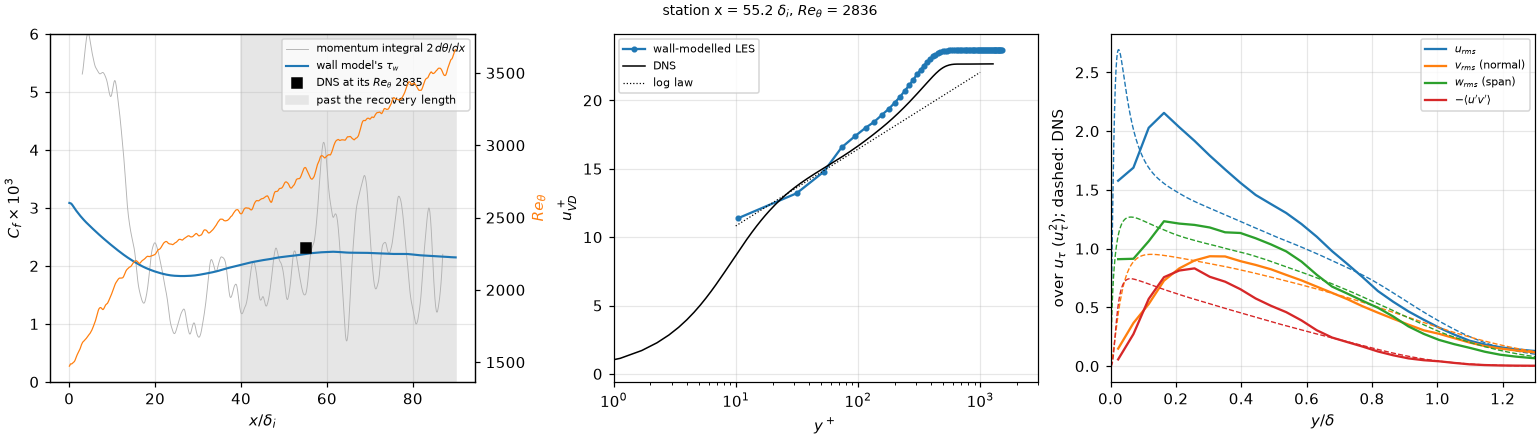
Left:
| At | LES | DNS |
|---|---|---|
| 2.21e-3 (the two halves of the window 2.19e-3, 2.22e-3) | 2.31e-3 | |
| 1.56e-3 | ||
| 4.08 | 4.10 (its profile: 4.22) | |
| 13.1, 17.5, 19.8 | 13.6, 16.7, 18.8 | |
| 2.06, 0.81, 1.22 | 1.49, 0.93, 1.12 | |
| 0.80, 0.50 | 0.62, 0.37 |
What it shows.
within 4.4 % of the DNS at its , with the setting that matched the Mach 3 channel. The two halves of the averaging window differ by 1.1 %. Most of the 4.4 % is the inflow's recovery, not the plateau: farther downstream, at – , is within 1.6–0.4 % of the DNS's value scaled as , and at it is 0.2 % at the station (resolution). - The inflow recovers by
. The layer reaches the DNS's at , against 53 in the DNS. falls from at the inlet to at , the adaptation of the synthetic eddies, then rises to a plateau of from . That matches the recovery length of a digital filter at this Mach number (Huang, Duan & Choudhari 2022). - The momentum integral does not measure
here. Fitted over , swings between and along on the same averaged data, and is % at the station. - The log layer sits 0.9–1.0 above the DNS in
, and peaks too high, the near-wall streaks of a coarse LES. The resolved in the outer layer is above the DNS's. At the log layer, and move toward the DNS. is the DNS's within 1 % (4.08), taken against the local free stream as the DNS takes it.
The flow
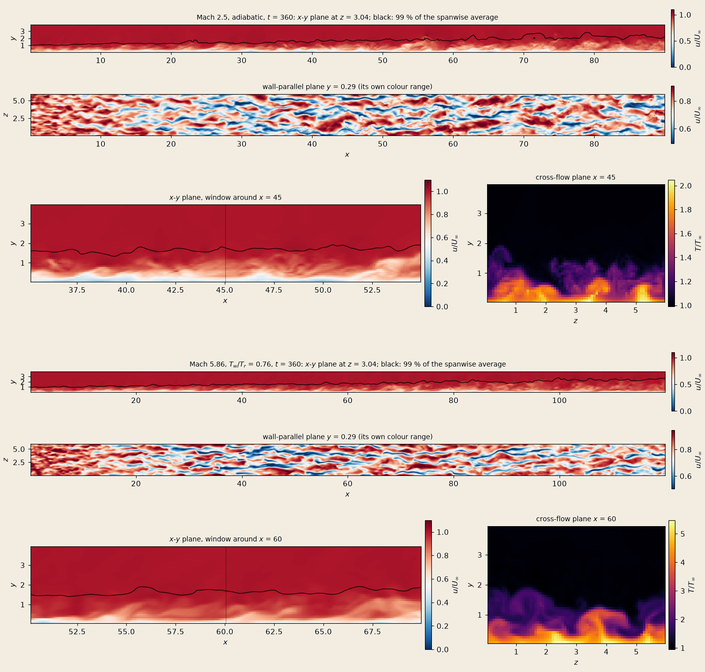
The last checkpoint of the Mach 2.5 run (top block, make_doc_figures.py --only tbl-fields.
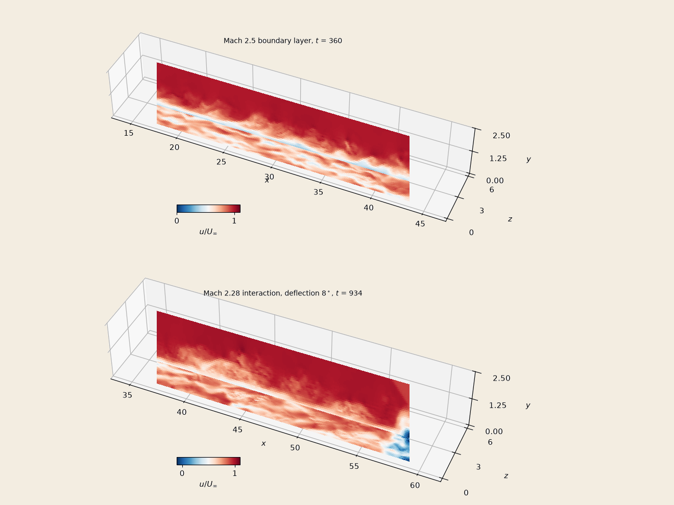
The same planes as the faces of a cutaway, make_doc_figures.py --only tbl-3d.
- The streaks at
( ) are outer-scaled. The first minimum of the spanwise correlation of puts them – apart at Mach 2.5 and – at Mach 5.86, about one , the same near the inflow ( ) and downstream ( ). At the first cell is , about 26 wall units at ; the near-wall cycle is the wall model's, as in the channel. - The edge of the layer is corrugated by bulges of about
in length. The cold-wall layer's cross-section shows the hot fluid near the wall (up to ) lifted in ejections; at Mach 2.5 the near-wall temperature is the adiabatic .
Resolution: Mach 2.5 at
| Setup | |
|---|---|
| grid | the same |
| wall | the matching point still the 3rd cell, so |
| inflow | the filter's node spacing the new |
| run | tbl_cases_t37_r16.txt, 35264 steps, 30 checkpoints of |
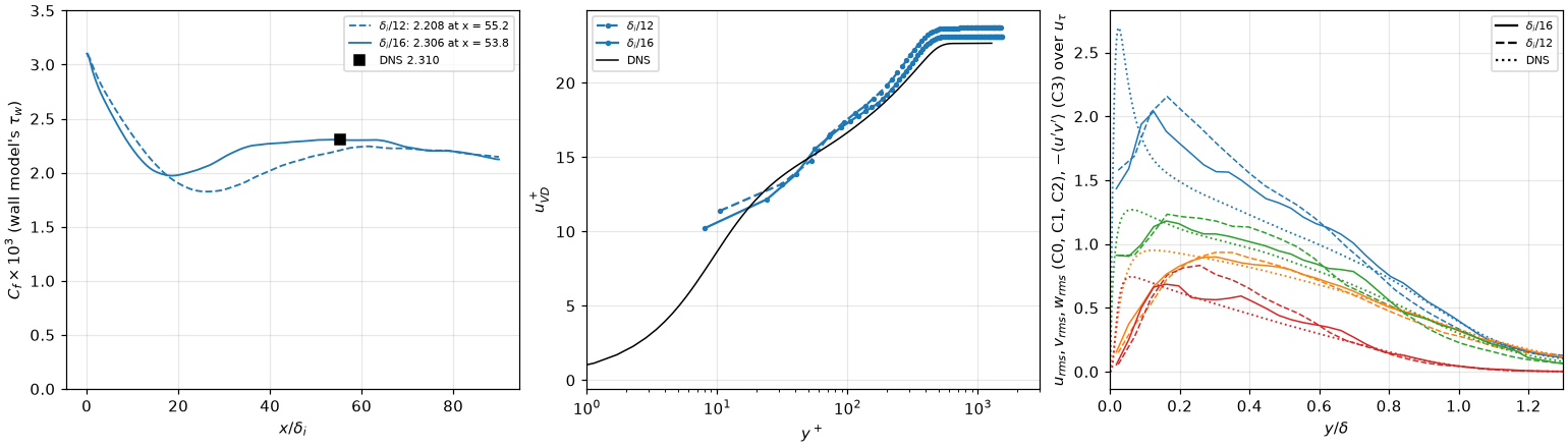
Left:
| DNS | |||
|---|---|---|---|
| 2.208e-3 (halves 2.195e-3, 2.220e-3) | 2.306e-3 (halves 2.299e-3, 2.312e-3) | 2.310e-3 | |
| −12.0, −3.9, −1.6, −0.9, −0.4 % | −3.6, −0.3, +1.0, +0.7, −0.5 % | ||
| 4.08 | 4.23 | 4.10 (its profile: 4.22) | |
| 13.1, 17.5, 19.8 | 12.8, 17.3, 19.2 | 13.6, 16.7, 18.8 | |
| 2.06, 0.81, 1.22 | 1.79, 0.83, 1.16 | 1.49, 0.93, 1.12 | |
| 0.80, 0.50 | 0.66, 0.43 | 0.62, 0.37 |
What it shows.
is grid-converged once the layer has recovered. Downstream of ( ) the two grids agree with each other and with the DNS's scaled as within 1–2 %. The scaling is an approximation (the DNS file holds one station), so these figures carry its error too. - The finer grid shortens the inflow's recovery. The
dip after the inlet ends by at , against – at : the % at the DNS station of the run is mostly the layer still recovering. At the station is past it, and is %; the halves of the window differ by 0.6 %. - The near-wall and log-layer statistics converge toward the DNS: the
peak at from 2.06 to 1.79, from 0.80 to 0.66, the log-layer offset in at from +1.0 to +0.4. is the DNS's on both grids (4.08, 4.23, against 4.10) taken against the local free stream (the shape factor).
The shape factor and the free stream
The DNS's profiles are normalised by its free stream at the station, and are 1 there. The run's free stream is not the nominal one: the layer thickens downstream and turns the supersonic stream over it, a weak compression of order tbl_oracle.py compare therefore takes
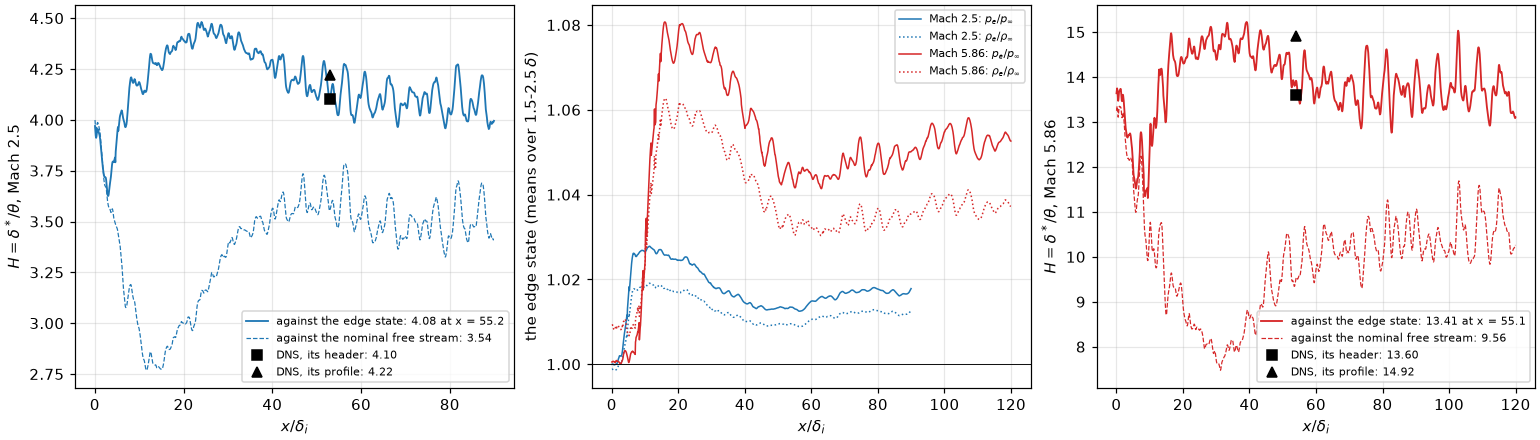
Left and right:
What it shows.
- The free stream is compressed. At Mach 2.5
rises to 1.027 at and is 1.013 at the station, 1.009; at Mach 5.86 1.08 and 1.042. Integrated to the top of the box ( , more than ), the denser stream over the layer takes 0.5 off at Mach 2.5 and 4 at Mach 5.86. The dip of the nominal to 2.8 at is the compression's peak, not the layer. - Against the edge state
is the DNS's: 4.08 at Mach 2.5 (4.10, its profile 4.22), 13.4 at Mach 5.86 (13.6, its profile 14.9). Taken over – , – or – , the edge moves it by 0.04 at Mach 2.5.
Sensitivity: five settings at
The Mach 2.5 case with one setting changed in each run. Same averaging, 33–35 checkpoints of
| Run | Change from the baseline | Cases file |
|---|---|---|
| lengths | the filter's integral lengths from | tbl_cases_t37_hdef.txt |
| span | span doubled to | tbl_cases_t37_hdef.txt |
| WALE, Vreman | [turbulence] sgs_model = wale, vreman, default constants | tbl_cases_t37_sgs.txt |
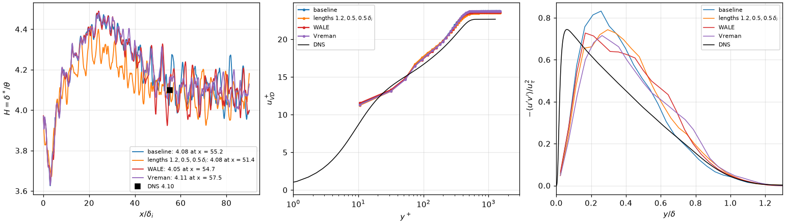
Four of the runs (the span of
| At | baseline | lengths | span | WALE | Vreman | DNS |
|---|---|---|---|---|---|---|
| station | 55.2 | 51.4 | 54.6 | 54.7 | 57.5 | 53 |
| 4.08 | 4.08 | 4.11 | 4.05 | 4.11 | 4.10 (its profile: 4.22) | |
| 2.208e-3 (−4.4 %) | 2.248e-3 (−2.7 %) | 2.205e-3 (−4.6 %) | 2.235e-3 (−3.3 %) | 2.206e-3 (−4.5 %) | 2.310e-3 | |
| 13.1, 17.5, 19.8 | 13.0, 17.7, 19.8 | 13.0, 17.5, 19.9 | 13.2, 17.4, 19.7 | 13.0, 17.5, 19.7 | 13.6, 16.7, 18.8 | |
| 2.06, 0.81, 1.22 | 1.97, 0.75, 1.15 | 2.08, 0.79, 1.22 | 1.97, 0.76, 1.19 | 1.94, 0.74, 1.27 | 1.49, 0.93, 1.12 | |
| 0.80, 0.50 | 0.66, 0.57 | 0.74, 0.56 | 0.72, 0.55 | 0.66, 0.49 | 0.62, 0.37 |
What it shows.
- None of the settings changes the layer much.
stays within 0.06 of the DNS's header value, within 2 % of the baseline's; longer integral lengths shorten the inflow's recovery a little (the layer reaches at , −2.7 %), as does. - The subgrid model is active, and does not matter at this grid. WALE's eddy viscosity, computed from a checkpoint, is about 1.5 times the molecular one over
– and 0.4 at the edge. - What is left is in the stresses, not in the mean: the outer
is 0.49–0.57 at against 0.37 in the DNS, and the near-wall peak 1.9–2.1 against 1.5. At both move toward the DNS (resolution).
Mach 5.86, cold wall
Case M6Tw076 of the same DNS: Mach 5.86, a cold wall (
| Setup | |
|---|---|
| box, cells | |
| gas | tbl_oracle.py compare --re-inf) |
| gas, Sutherland run | viscosity_law = sutherland (#121 S1), tbl_cases_t37_hdef.txt, 29 checkpoints) |
| wall, inflow, scheme | as at Mach 2.5 |
| run | tbl_cases_t37_m6.txt, to |
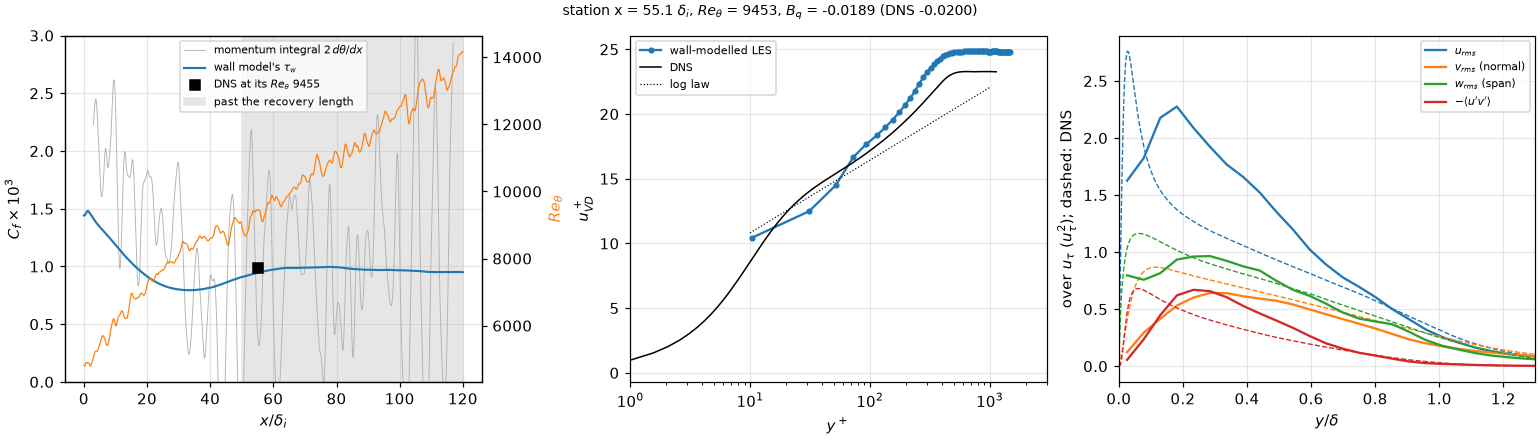
The panels of the Mach 2.5 figure; the title adds
| At | LES | LES, Sutherland | DNS |
|---|---|---|---|
| 9.47e-4 (the two halves of the window 9.70e-4, 9.25e-4); | 9.51e-4; | 9.84e-4 | |
| −0.0189 (halves −0.0191, −0.0187); | −0.0190 | −0.02 (one significant figure) | |
| 1.61 | 1.61 | 1.72 | |
| 13.41 | 13.71 | 13.6 (its profile: 14.9) | |
| 12.4, 17.9, 20.8 | 12.4, 17.9, 20.6 | 13.9, 17.2, 19.5 | |
| 2.21, 0.56, 0.94 | 2.24, 0.55, 0.90 | 1.33, 0.82, 0.99 | |
| 0.64, 0.39 | 0.65, 0.35 | 0.49, 0.25 |
What it shows.
within 3.8 % of the DNS at its , with no change of the wall-model setting from Mach 2.5; past the plateau is 0.7 % below. agrees to the precision of the reference. The DNS file gives , one significant figure, and the run gives 0.0189 at the station, 0.0194 on the plateau. drifts by 4.6 % between the two halves of the window; by 0.4 %. The layer itself changes slowly over the window, and the wall model's heat flux follows its friction. 180 time units are 1.5 flow-throughs of this box, so the figure carries about %. - The inflow recovers by
– , farther than at Mach 2.5 (50): falls from at the inlet to at , then rises to its plateau. The layer reaches the DNS's at , against 54 in the DNS. is the DNS's against the edge state (13.4; the header 13.6, its profile 14.9): the free stream over this layer is compressed by 4 % (the shape factor). - The stresses have the Mach 2.5 faults, larger.
is 6 % thin; peaks at 1.7 times the DNS's at , and is 1.5 below the DNS at (the first cells under the matching point) and 0.7–1.3 above it at – . At the layer of has about 20 cells across ; at Mach 2.5 a finer grid moves the log layer and the stresses toward the DNS (resolution). - Sutherland's law with the DNS's Reynolds number changes little. The power-law viscosity, matched at the wall, is 1.41 times the DNS's in the free stream; Sutherland's law removes that:
13.71 against 13.41, −3.4 % against −3.8 % at the station, the plateau 9.80e-4, −0.0190. - The momentum integral does not measure
here either ( % at the station, negative in places).
The wall model fed with the resolved convection
The zero-gradient check of the convection-fed model before it is used in the shock interaction (turbulence): fed with the instantaneous resolved convection it raised the
| Setup | |
|---|---|
| runs | the Mach 2.5 case above (m2p5-wm-l90, the baseline, statistics wall_model_pressure_gradient (filter 10), wall_model_convection and wall_model_resolved_stress; statistics over the 27 checkpoints of tbl_oracle.py compare --t0 400); one node, 4 A30, about 3 h each |
| rs | the resolved shear stress removed from the forcing, the velocity scale of the eddy viscosity $\sqrt{( |
| rs2 | the key's model: the resolved stress removed and the velocity scale $\sqrt{ |
| a priori | wmf_apriori.py on the filtered averages of rs's .wmf (77760 wall columns): the model's variants on the same samples |
| f50, f100 | the slow forcing: rs restarted at wall_model_velocity_scale = sum (the scale wall_model_pressure_gradient_filter, against rs's 10); statistics over the 34 checkpoints of |
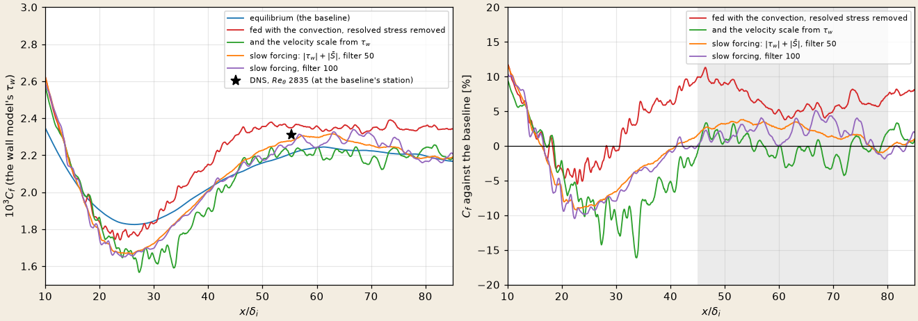
Left: make_doc_figures.py --only tbl-convection.
| baseline | rs | rs2 | f50 | f100 | |
|---|---|---|---|---|---|
| the same, range along | |||||
| a priori, mean | |
|---|---|
| the pressure gradient alone | |
| fed with the convection | |
| and the resolved stress removed | |
| and the velocity scale from | |
| the resolved stress removed, fed the span-mean forcing |
- Removing the resolved stress is not enough. The filtered forcing at the sample fluctuates as much as
(rms against a mean of ), and in the velocity scale averages far above the mean forcing: the eddy viscosity grows and with it (rs, +6.6 % in the run, +12.4 % a priori). - With the forcing out of the eddy viscosity the layer is the baseline's. rs2's
is the baseline's within 0.3 % over the developed stretch and % against the DNS at the station (the baseline %), as the a priori % predicted: the gate passes. - Where the layer recovers from the inflow it is lower. Over
, behind the digital-filter inflow, rs2's is 8.6 % below the baseline's: there the resolved convection does not vanish, and the model answers to it. The DNS station lies beyond, so which of the two is right there is not measured. - The slow forcing keeps the layer within about 2 %. With the scale
(which keeps the eddy viscosity under an adverse gradient, interaction) and a forcing filtered over 50 or 100 instead of 10, the developed stretch sits and % above the baseline, against rs's %: the filter does most of the work between 10 and 50, little beyond (the a priori limit of an infinite filter, and %, is near). With the criterion of 2 % fixed before the runs, f100 passes and f50 falls 0.2 % short, a difference within the scatter along (the first 20 checkpoints of the same window gave and %). Both move the station toward the DNS ( , % against the baseline's %).
The viscosity coupling
The zero-gradient gate of wall_model_coupling = viscosity (turbulence, #126): the no-slip condition kept and the face stress the larger of the first cell's molecular no-slip stress and the model's, along the first cell's wall-parallel velocity. In the shock interaction it separates the wall stress in the mean (S4l). Criteria fixed before the runs:
| Setup | |
|---|---|
| runs | rs's state at wall_model_coupling = viscosity, ctrl with the default flux; statistics over the 33 and 34 checkpoints of tbl_oracle.py compare --t0 720); one prod-gn job, a run per node (4 A30), 4 h |
| grid | the baseline's: |
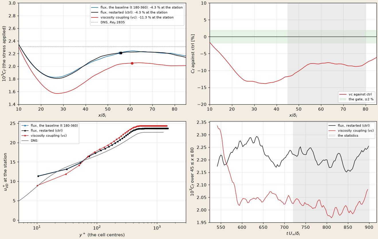
Top: make_doc_figures.py --only tbl-coupling.
| baseline | ctrl, flux | vc, viscosity | |
|---|---|---|---|
| 4.10 | 4.22 | ||
| 11.3, 13.1, 14.7 | 8.9, 11.9, 14.1 | ||
| molecular no-slip stress of the first cell against the applied, | 1.08 | 0.88 |
- The gate fails: the coupling lowers the zero-gradient stress by 9 %. Over the developed stretch vc's
is 8.7 % below ctrl's, and % against the DNS at the station; ctrl reproduces the baseline ( %). The drop settles within about 60 time units of the restart and holds over the window (bottom right), so it is the coupling's, not a transient. - How: the maximum drags the first cell down to its no-slip velocity, and the sample with it. Under the flux coupling the first cell runs at
at , faster than the DNS's 8.9 there: its no-slip stress would be 1.08 times the model's. Switched to the viscosity coupling, the maximum takes that larger stress (vc's first rises above ctrl's, bottom right), the first cell slows to , the DNS's value within 2 %, and the cells above it slow too ( at against the DNS's 13.6). The model reads the slower velocity at and returns a lower , which the face then applies wherever it exceeds the molecular one. - De Vanna et al. (2022) reproduce the model's stress exactly with the resolved gradient (an effective wall viscosity
, no lower bound stated); the lower bound here, which keeps the molecular stress where the wall is resolved, is what lets the first cell's no-slip gradient win. The variant without it, the model's magnitude along the first cell's velocity, is not tested.
Recycling inflow
The recovery gate of the inflow-recycling face (turbulence, #121 S5): the digital filter's layer needs about
| Setup | |
|---|---|
| run | rs's state at inflow-recycling at station make_tbl.py --inflow recycling --rr-x 20: thickness ratio 1.3305, tbl_oracle.py compare --t0 720); one prod-gn node (4 A30), 4 h 36 min |
| grid | the baseline's: |
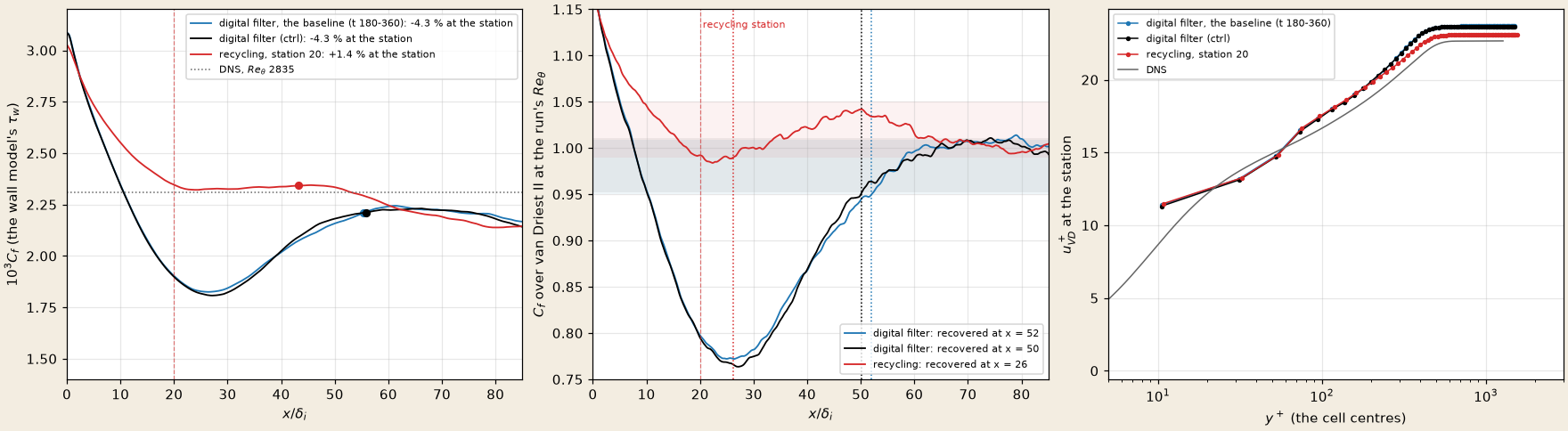
Left: make_doc_figures.py --only tbl-recycling.
| ctrl, digital filter | rr, recycling | |
|---|---|---|
| recovery length, 3 % of the run's own mean over | ||
| deepest departure beyond | ||
| first | 53, 55 | 10, 55 |
| 1.004 | 1.005 | |
| station ( | 55.9, | 43.3, |
| 4.10; 1469 | 3.98; 1518 | |
| 13.0, 17.5, 19.9 | 13.1, 17.6, 19.8 | |
| 1.91, 0.81, 1.23 | 1.90, 0.74, 1.09 | |
| wall time per step (whole run, one node; ctrl ran beside vc on a second node) | 0.61 s | 0.63 s (+3 %) |
- Recycling removes the digital filter's dip. Beyond the station the ratio never falls more than 2 % below the level both digital-filter runs reach downstream, against 24 % at
under the digital filter; it is within 4 % of that level from , the digital filter from . The gate's measure gives against 50, half. - The 3 % criterion against the common level does not separate them: both enter at
. The recycled layer runs up to 3.8 % above the downstream level (more than 3 % over , more than 2 % over ) before it joins it; the gate's measure, which takes each run's own mean (1.020 for rr), absorbs that bump into its band. Which of the two references is right is a choice of criterion; the departure (4 % against 24 %) is not. - The station comparison is not a better wall model. rr's
% and ctrl's % against the DNS are each run's departure from the same downstream level ( and %), taken where falls: inside rr's bump ( ), at the end of ctrl's recovery ( ). The level itself, carried to by van Driest II, is % against the DNS for both. The profiles at the station agree within 0.1 in ; the recycled layer's and at are 9 and 11 % lower than ctrl's. - The cause of the bump is not identified. The face's layer is 4 % thicker than the table's (
1.04 against 1.00, 1518 against 1469): the correlation's ratios, fixed for the run, against the layer's own growth to the station are the first suspect, not tested. - The cost is 3 %, the whole run's wall time per step against ctrl's on another node of the same kind; the first minutes ran at 0.82 s per step, a start-up transient.
Not done
- The matching height at fixed grid; the outer-layer and near-wall stresses at
. at Mach 5.86; a longer averaging window at Mach 5.86. and the station against the edge state: they use the nominal free stream. - Mean profiles against the DNS beyond the station.
- The viscosity coupling without the lower bound on the wall's subgrid viscosity (the model's stress along the first cell's velocity).
- Recycling: the bump above the downstream level (ratios measured from the run against the correlation's), the station's distance, the recycling frequency
in the incoming layer, a longer window.