

Appearance
Shock/boundary-layer interaction
| ID | Milestone | Type | Legs | Backends | Figure |
|---|---|---|---|---|---|
— (campaign tbl_cases_s4.txt) | #121 · S4b–S4l | P | none (the pressure-gradient key: wm12) | FNL | yes |
Case and scope
The interaction of the IUSTI experiment (Dupont, Haddad & Debiève 2006, JFM 559) as computed by the STREAmS DNS (Bernardini, Modesti, Salvadore & Pirozzoli 2021, CPC, Fig. 7): Mach 2.28, an oblique shock of
Setup
| Setup | |
|---|---|
| box, cells | |
| shock | |
| gas | |
| wall, inflow, scheme | wall-modelled at reference/tbl_m2p28_profile.txt); hybrid-kep-weno |
| run | tbl_cases_s4.txt, to sbli_oracle.py compare --t0 300) |
| references | the DNS wall pressure and the IUSTI points of STREAmS Fig. 7a, whose reference/sbli_m2p28_*, error in the headers) |
sbli_oracle.py takes
Results
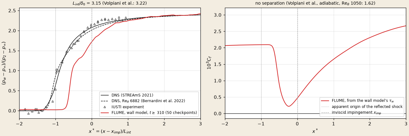
Left: the mean wall pressure make_doc_figures.py --only sbli.
| FLUME, wall model | Reference | |
|---|---|---|
| 5247 / 4667 | about 5000 (DNS, experiment) | |
| reflected shock: angle to the wall | ||
| 3.15 | 3.22, Volpiani et al. (DNS, | |
| separation: | 0, | 1.62, Volpiani et al., |
| 0.02, 1.12, 1.72, 2.09, 2.24, 2.37 | DNS: 0.64, 1.75, 2.07, 2.22, 2.29, 2.36; at | |
| Souverein | 1.93, 1.20 |
The flow
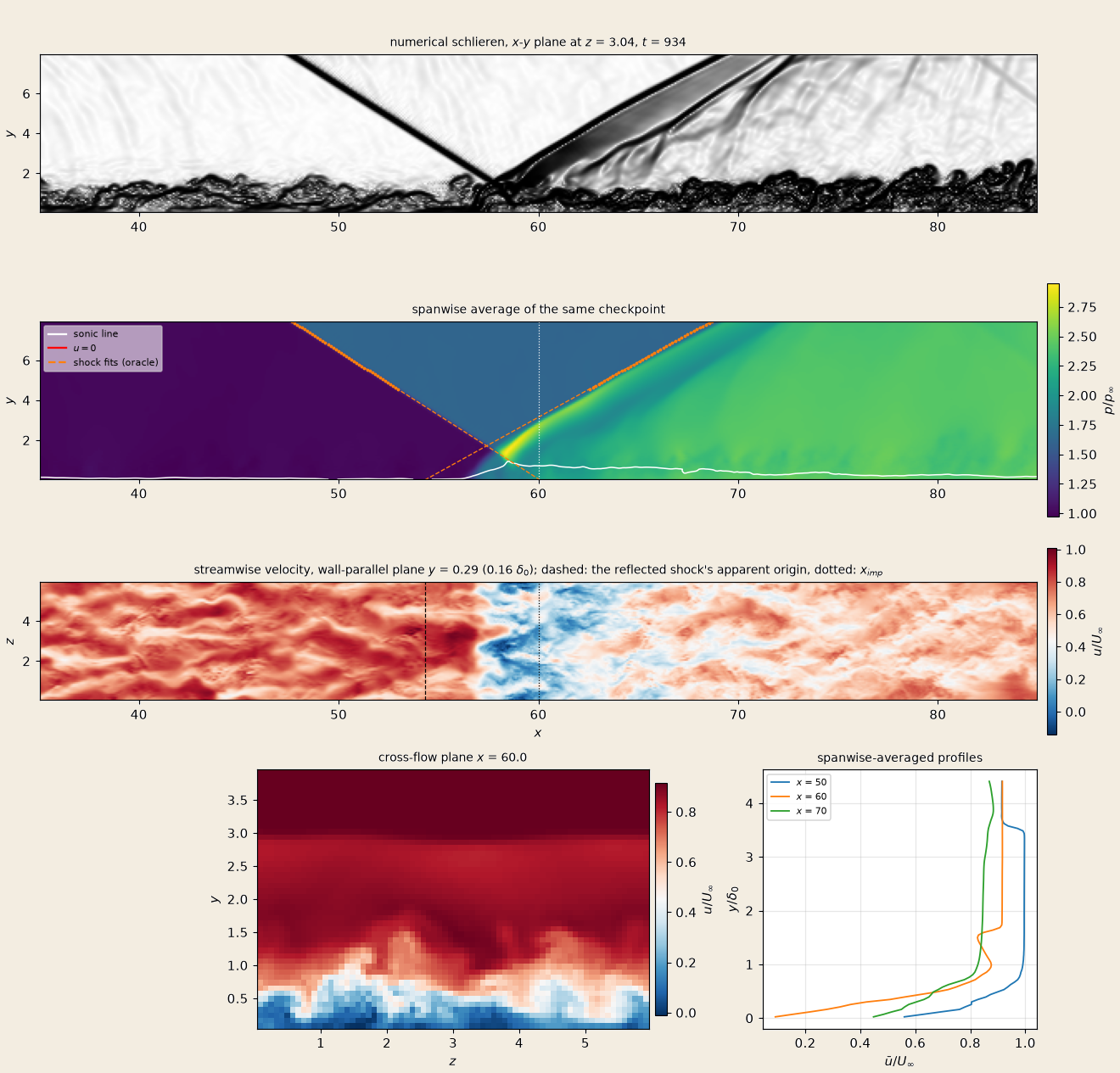
One checkpoint (make_doc_figures.py --only sbli-fields.
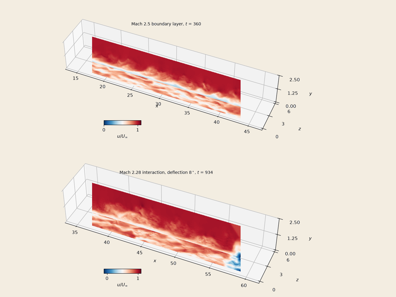
A cutaway, make_doc_figures.py --only tbl-3d.
What it shows
- The interaction length is right.
against 3.22 in the DNS of Volpiani et al. (2018, at ), and the reflected shock leaves at , under the inviscid angle. The downstream pressure plateau is the DNS's within 4 % ( ). - The mean flow does not separate.
dips to and recovers; the DNS, the experiment and Volpiani et al. have a bubble. It comes close: in one checkpoint the spanwise-averaged of the first cell falls to between and 65, and the wall-parallel plane at has patches of (down to ) between and 61.9. The wall model's follows the velocity at its matching height, the 3rd cell, whose mean stays positive. - The wall pressure rises late. It starts at
and is half-way to at ; the DNS are there at and , in the separation that the DNS have and this run has not. Downstream of the impingement the pressure is the DNS's within 4 %. (The first version of this page read the reference's from , as the STREAmS paper's text says, and found the rise early: the figure measures it from the reflected shock, below.) - Two candidate causes of the missing separation, tested since. The equilibrium model has no pressure-gradient term, and it computes
from the velocity at the 3rd cell, or above the wall, which the near-wall deceleration under the adverse gradient reaches late. S4c halves the matching height: the dip of halves, the mean does not separate. S4d adds the pressure gradient: a bubble of , the compression unchanged.
A refined wall grid under the interaction
Run S4c is the S4b case with one more level, 2:1, under the interaction (tbl_cases_s4c.txt). The wall model and its matching point (the 3rd cell) are unchanged, so in the refined box the matching height halves with the cells. A bubble in this run points at the near-wall grid; none points at the equilibrium model.
| Setup | |
|---|---|
| grid | S4b's box and base grid (make_tbl.py --refine-box 30,75,2.5 refines a block when its centre is inside |
| matching height | the 3rd cell: |
| seams | the box's upstream face is at |
| start | from wm3 verifies). The cost is S4b's |
| run | to |
| oracle | sbli_oracle.py compare --t0 300: tbl_oracle.averages maps the two levels onto the fine grid (coarse cells repeated); field_slices.py cuts the planes on the fine grid the same way |
Cost on two nodes
The first FNL run of FLUME across two medooza nodes. S4b ran 64 blocks on 4 A30 (one node) at 0.74 s per step; S4c runs 120 blocks of the same size on 8 A30 at 0.95 s per step at the start and 0.98 at
The step was slower because of the partition, not the network. The 120 blocks landed 20/13/19/17/13/19/19/0 on the 8 ranks: one GPU held no block, and the busiest held 20 against an even 15, which made each step 1.33 times slower than an even split. mpi_redistribute then walked the blocks greedily and kept the 8 siblings of a refined parent together; a model of the routine reproduces that split exactly (#123). A static grid is now balanced by block count ([amr] balance_static, on by default: 15 per rank on this tree), and a runtime regrid by a min-max split of the sibling sets (busiest 18). Evenly split, the step would take about 0.71 s, so the run would need about 13.5 hours instead of 18.
Results
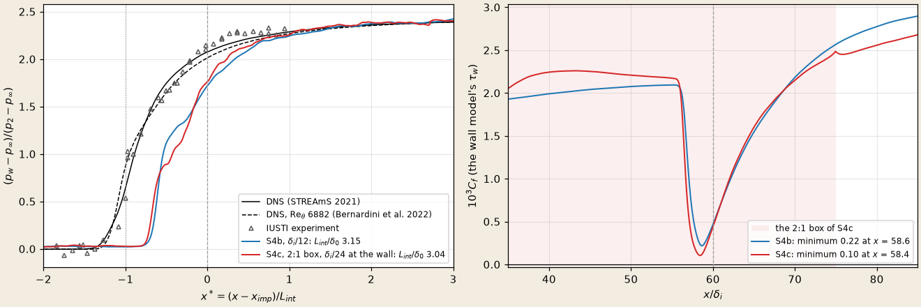
Left: the mean wall pressure of S4b and S4c against the DNS and the experiment. Right: make_doc_figures.py --only sbli-refined.
The statistics are the span and the 21 checkpoints of sbli_oracle.py compare --t0 300); S4b's column repeats the table above.
| S4c, 2:1 box | S4b | |
|---|---|---|
| 5314; | 5247; | |
| reflected shock: angle to the wall | ||
| 3.04 | 3.15 (DNS of Volpiani et al.: 3.22) | |
| separation: | 0, | 0, minimum |
| 0.89, 1.76, 2.14, 2.26, 2.39 | 1.12, 1.72, 2.09, 2.24, 2.37 (DNS: 1.75, 2.07, 2.22, 2.29, 2.36) | |
| S4b's within 0.4 % | ||
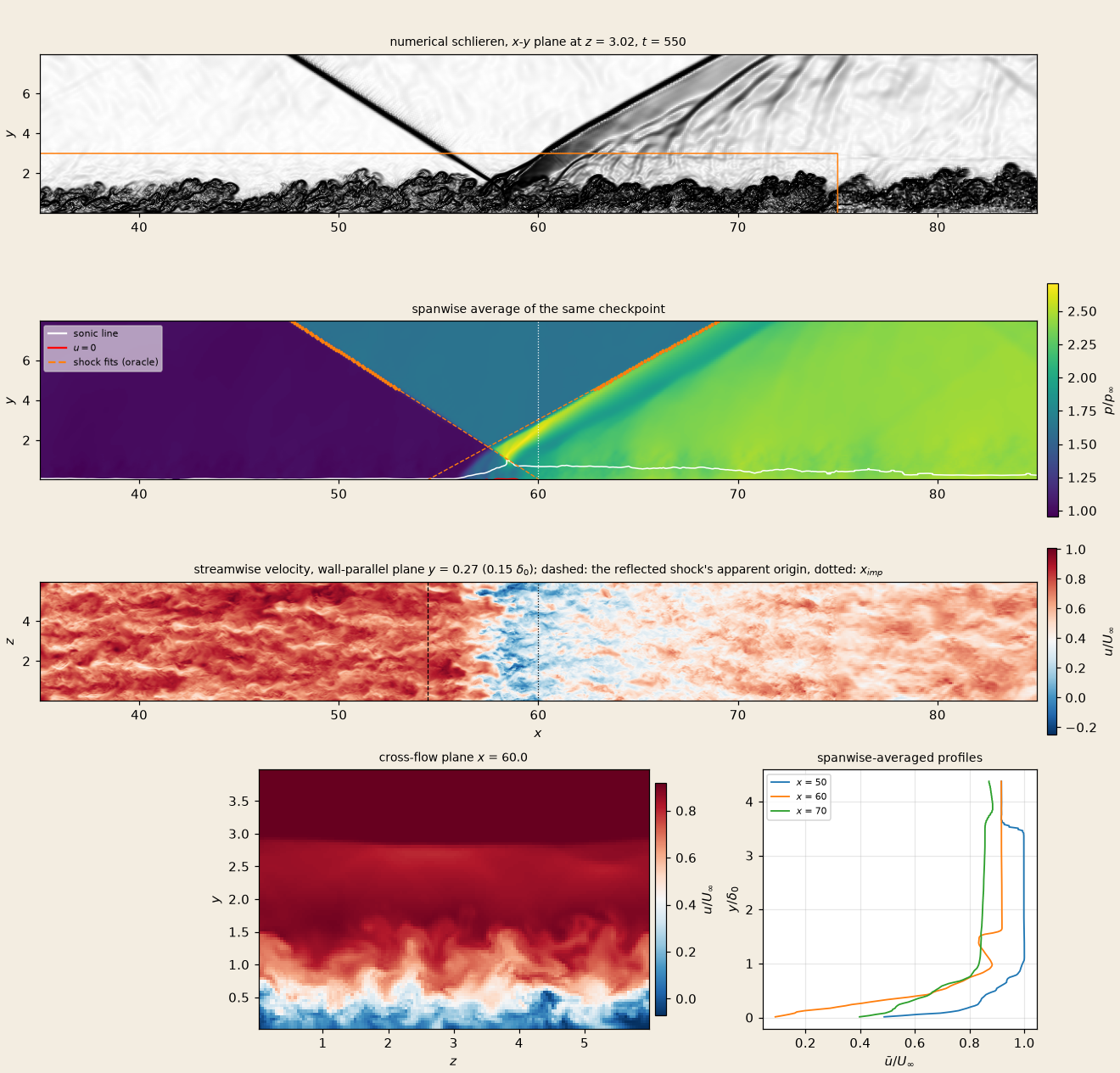
The panels of the flow for S4c at make_doc_figures.py --only sbli-refined-fields.
- The finer near-wall grid does not open a mean bubble. Halving the matching height halves the dip of
, at the same place, and the mean stays positive. In single checkpoints the flow at the wall reverses in patches: at the spanwise-averaged of the first cells is negative over a short stretch near (the red line), and the cross-flow plane at has reversed cells along the wall. The reversal is intermittent; the mean has none. - The interaction length shrinks slightly, 3.04 against 3.15, and the rise is shallower (
at against S4b's and the DNS's ), its onset unchanged (below): the shape of the interaction is S4b's. - The zero-pressure-gradient layer depends on the matching height. Outside the box
is S4b's; inside it, after an adjustment over about behind the 2:1 face, it is 10 % higher before the interaction. The equilibrium model's follows the velocity at its matching point, and that point moved from to (the log-layer mismatch of Kawai & Larsson 2012). A matching height fixed in , not in cells, would keep the two levels consistent; it does, within 1.7 % (S4k). - What remains is the model. The equilibrium model integrates a constant total stress across its layer, so its
turns negative only where the velocity at the matching height reverses on average. With the matching point at it does not; the pressure-gradient term, which lets reverse under a strong adverse gradient while the matching velocity is still positive, was tested next (below): a bubble of , a quarter of the DNS's.
The matching height fixed: S4k
The configuration of Kawai & Larsson (2012) and of Hoy & Bermejo-Moreno (2022) on this grid: the matching height fixed in wall_model_height sbli_oracle.py compare --t0 650). Criteria fixed before the run: (a)
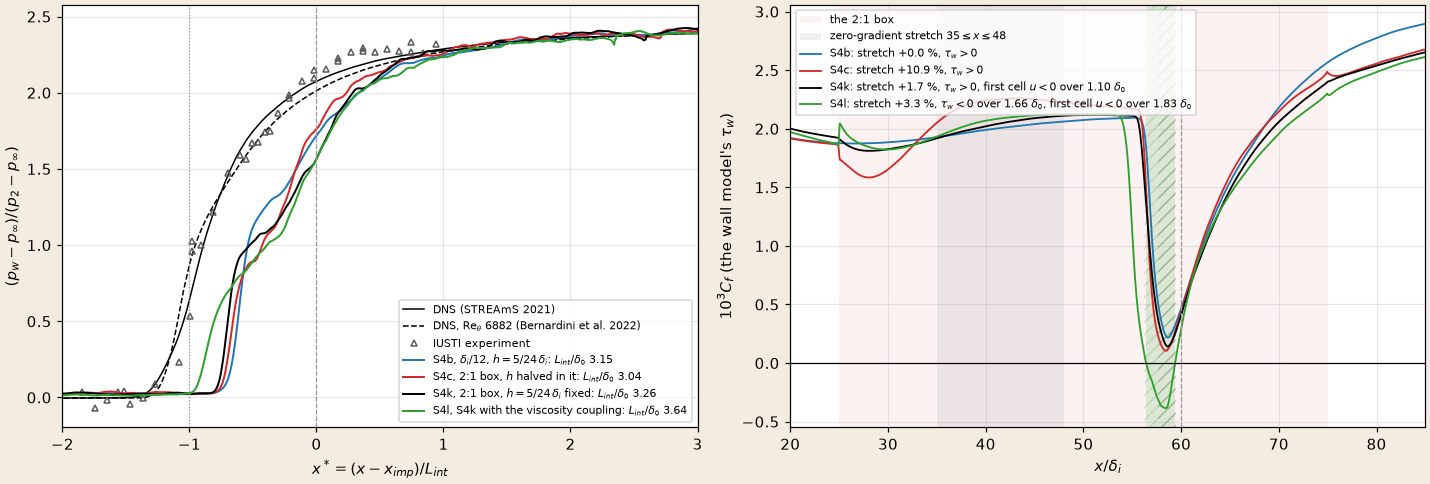
Left: the mean wall pressure of S4b, S4c and S4k against the DNS and the experiment. Right: make_doc_figures.py --only sbli-fixed-h.
| S4k, 2:1 box, | S4c, 2:1 box, | S4b | DNS, | |
|---|---|---|---|---|
| 5253; 1.783 | 5314; 1.824 | 5247; 1.807 | ||
| +1.7 % | +10.9 % | |||
| +4.2, +2.2, | ||||
| 3.26 | 3.04 | 3.15 | 3.30 | |
| 0; 0.14 at | 0; 0.10 at | 0; 0.22 at | 2.16 ( | |
| time-mean | none | none | ||
| 5 % / 50 % of the rise, | 2.58 / 2.28 | 2.33 / 2.00 | 2.34 / 1.96 | 4.13 / 3.60 |
| 1.02, 1.57, 2.11, 2.28, 2.39 | 0.89, 1.76, 2.14, 2.26, 2.39 | 1.12, 1.72, 2.09, 2.24, 2.37 | 1.75, 2.07, 2.22, 2.29, 2.36 | |
| reversed area per unit span, mean (max), | 0.115 (0.138) | 0.069 (0.084) | 0.068 (0.142) | |
| first / third cells reversed in the window | 23.4 % / 12.6 % | 14.5 % / 8.7 % | 9.5 % / 5.1 % |
The two refined runs count fine cells, S4b coarse ones: the reversed fractions compare S4k with S4c.
- (a) passes: the matching height fixed in
keeps the refined layer on S4b's. Over is 1.7 % above S4b's, against S4c's 10.9 %: the log-layer mismatch of the halved matching height was S4c's drift. One difference outside the box was not planned: there falls on the 3rd cell's centre, the sample weight comes out instead of 0, and the eddy viscosity below , which skips the sample cell only when the weight is exactly 0, also enters the 3rd cell ( sample_cells,adam_flume_wall_model_library.F90). Upstream of the boxis then 4.2 % above S4b's, and the layer entering the box carries that. sample_cellsnow snaps a weight belowto 0, so a matching height on a cell centre is that cell; S4k and S4l (whose coarse region has the same defect) were not run again. - (b) half passes: the resolved flow separates, the wall stress does not.
is the DNS's within 1.2 %, and the compression starts earlier than in S4b and S4c (still behind the DNS's). For the first time with the plain equilibrium model the time-mean of the first cell is negative, over (half the DNS's bubble, in its downstream half), and of the second over ; a quarter of the first cells are reversed in the window. The model's stays positive everywhere (minimum ): the bubble is about two fine cells tall, below the matching height, and the model, which sees only the flow at , keeps the positive of a forward flow over a reversed first cell. - So the remaining gap is the coupling. The face takes the model's
whatever the first cell does; a coupling through the wall viscosity with the no-slip condition kept (De Vanna et al. 2022), where the first cell sets the sign of the wall stress, is the next test (wall models in the literature): S4l (below).
The viscosity coupling: S4l
S4k with the model coupled through the wall viscosity, the no-slip condition kept (#126, wall_model_coupling = viscosity, turbulence): the face stress is the larger of the first cell's molecular no-slip stress and the model's, along the first cell's wall-parallel velocity, so a reversed first cell reverses the wall stress. Otherwise S4k's set-up (plain equilibrium model, sbli_oracle.py compare --t0 950). Criteria fixed before the run: (a)
| S4l, viscosity coupling | S4k, flux coupling | S4b | DNS, | |
|---|---|---|---|---|
| 5276; 1.757 | 5253; 1.783 | 5247; 1.807 | ||
| +3.3 % | +1.7 % | |||
| +2.7, | +4.2, | |||
| 3.64 | 3.26 | 3.15 | 3.30 | |
| 1.66, | 0 | 0 | 2.16 ( | |
| 0.14 at | 0.22 at | |||
| time-mean | 1.83, 1.14, | 1.10, | none | |
| 5 % / 50 % of the rise, | 3.48 / 2.93 | 2.58 / 2.28 | 2.34 / 1.96 | 4.13 / 3.60 |
| 0.89, 1.56, 2.09, 2.23, 2.35 | 1.02, 1.57, 2.11, 2.28, 2.39 | 1.12, 1.72, 2.09, 2.24, 2.37 | 1.75, 2.07, 2.22, 2.29, 2.36 | |
| sonic height at | 0.035 | 0.028 | 0.036 | |
| reversed area per unit span, mean (max), | 0.188 (0.217) | 0.115 (0.138) | 0.068 (0.142) | |
| first / third cells reversed in the window | 33.4 % / 18.9 % | 23.4 % / 12.6 % | 9.5 % / 5.1 % |
The green line of the figure above; the reversed flow per checkpoint in the reversal figure.
- (b) half passes: the wall stress separates in the mean, for the first time in this campaign.
over , three quarters of the DNS's bubble, at its downstream end ( to against to ). The compression starts earlier than S4k's (5 % of the rise ahead of , the DNS's 4.13), and the reversed flow grows: the first cells reverse in the mean over , a third of them in the window. overshoots: 3.64, 10.3 % above the DNS's 3.30, just outside the bound (Volpiani et al.'s 3.22 at ). - (a) fails: the stretch
is 3.3 % above S4b's (S4k's 1.7 %). In the box the first cell spans about 21 wall units. Under the flux coupling (S4k) its no-slip stress would be 1.14 times the applied one; under the viscosity coupling the maximum takes it, the first cell slows ( 0.409 against S4k's 0.488, the cells above less) and its no-slip stress falls to 0.94 of the applied. Two effects then pull apart: the maximum keeps picking the molecular stress whenever the first cell runs fast (with its rms of 17 % and a steady model stress, +3.8 %), and the slower sample lowers the model's stress. On the flat plate, with the sample 2.5 cells up, the second wins: % against the flux-coupled control (boundary layer); here, 5 fine cells up, the net is +1.6 % against S4k (a hypothesis: the model's own is not recorded apart from the applied one). The shift is also of the size of the scatter of S4k's own bands against S4b (from to +4.2 %). The sonic height at is the DNS's, against 0.036, where S4b's is 0.028. The stress also jumps at the 2:1 face ( , +10 % over about ), which the flux coupling does not: there the first cell enters the box at the coarse level's velocity, and the maximum takes its no-slip stress, as at the restart of the flat plate. - Behind the interaction the layer recovers more slowly (
8 to 10 % below S4b's over , S4k's 4 to 8 %).
The wall model with the pressure gradient
The equilibrium model has its wall_model_pressure_gradient (turbulence) the layer carries
A priori, on the mean fields
Before any run, the model was applied to the span and time averages of S4b and S4c: per sbli_oracle.py means and apriori; the port reproduces the Fortran solver to
| S4b, | S4c, | |
|---|---|---|
| the model without | ||
| without | nowhere (minimum | nowhere (minimum |
| with | ||
| with |
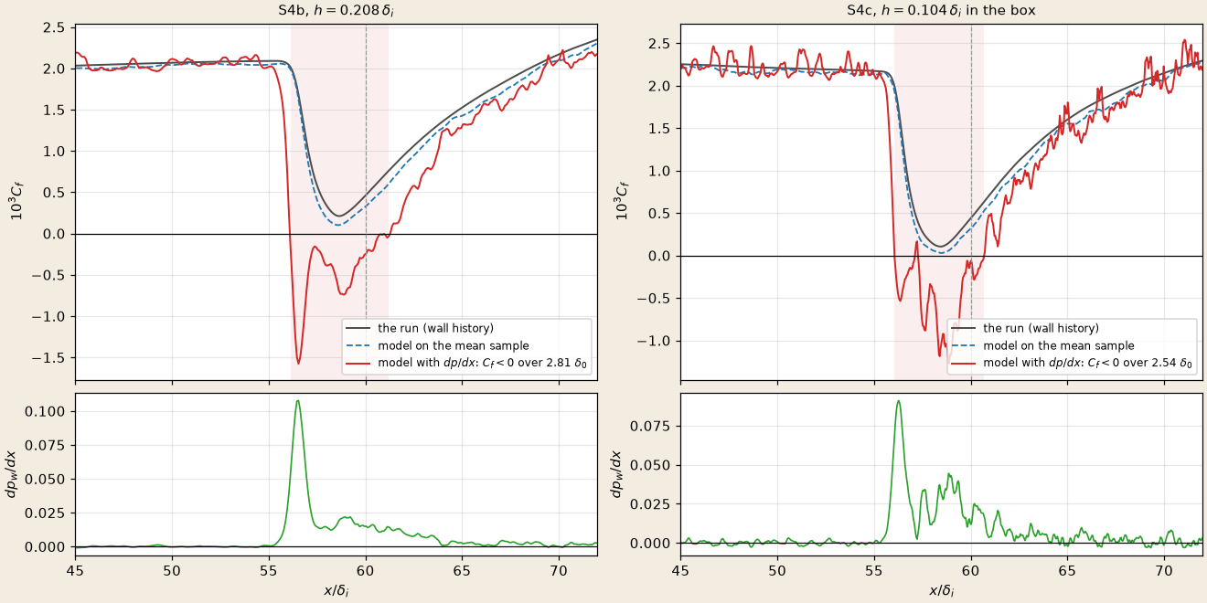
Top: make_doc_figures.py --only sbli-apriori.
- The term opens a bubble on both grids, 2.5–2.8
long, against 1.62 in the DNS of Volpiani et al. (at ). The model without it reproduces the runs' to 2 %, so the port is the run's model. - The term dominates there:
reaches about 70 in the bubble, far from the equilibrium layer the model assumes. The model keeps and drops the convective terms, which partly balance it in the wall layer: it can over-respond. - The mean field is the attached one. With a bubble the pressure rise spreads and
falls, so the run decides. - The instantaneous gradient cannot be used as it is. On a single checkpoint of S4b upstream of the interaction (
– ) the turbulent wall-pressure gradient has an rms of against a mean of , so has a median of 1.4, and the model with it raises the mean of the zero-pressure-gradient layer by 13 %. The run filters the gradient in time ( wall_model_pressure_gradient_filter).
The run
| Setup | |
|---|---|
| start | S4b's last state ([amr] balance_static = .false.) |
| model | wall_model_pressure_gradient = .true., wall_model_pressure_gradient_filter = 10 (about |
| run | to sbli_oracle.py compare --t0 1300); the input is S4b's make_tbl.py line with --restart --time-max 1450 --wm-pressure-gradient --wm-pg-filter 10 (no case file: a one-off restart) |
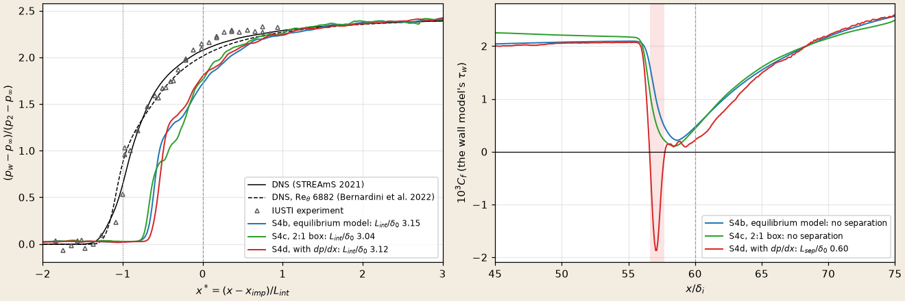
Left: the mean wall pressure of S4b, S4c and S4d against the DNS and the experiment; right: make_doc_figures.py --only sbli-pg.
| S4d, with | S4b | S4c, 2:1 box | |
|---|---|---|---|
| separation: | 0.60, | 0 | 0 |
| 3.12 | 3.15 | 3.04 | |
| reflected shock: angle to the wall | |||
| 0.95 | 1.12 | 0.89 | |
| 5288; 1.794 | 5247; 1.807 | 5314; 1.824 | |
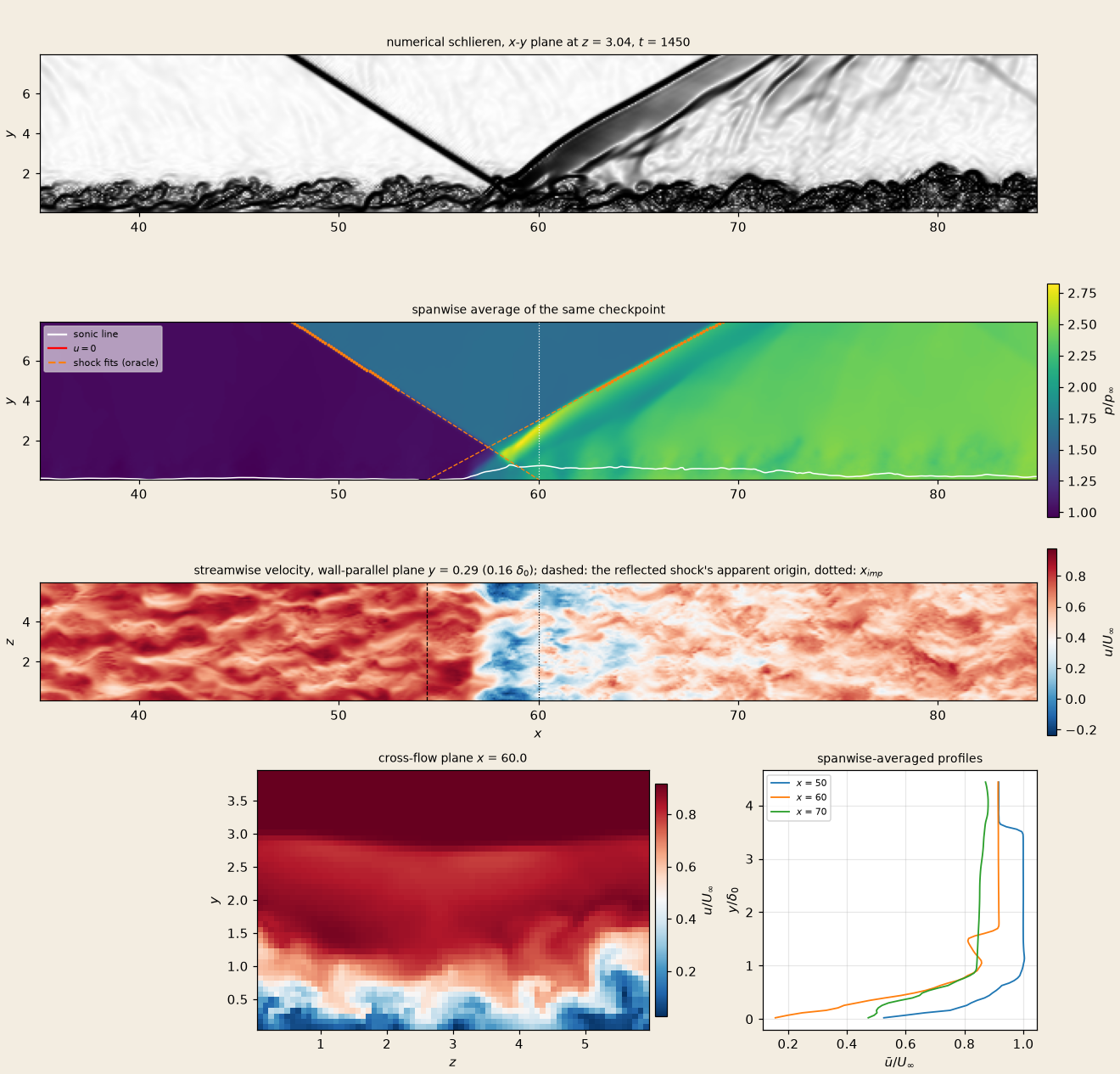
The panels of the flow for S4d at make_doc_figures.py --only sbli-pg-fields.
- The mean flow separates, for the first time in these runs:
is negative over at the foot of the reflected shock's compression, where the filtered gradient is largest, and reattaches before the impingement. The a priori test on the mean fields gave 2.5–2.8 for the same pressure field; the run's is a quarter of that, the gradient being filtered and the pressure rise unchanged. - The bubble is a quarter of the DNS's. The DNS at
separates from to , , ahead of the impingement as here; this one spans to , inside it. - The interaction does not change. The wall pressure still rises at
, half-way at against the DNS's , and is S4b's: the model's stress reverses, but the resolved flow above the matching height, which sets the pressure, does not. - What remains. The model keeps
and drops the convective terms (the known inconsistency): a non-equilibrium layer (the thin-boundary-layer equations with convection, or an integral model) is the next test of the wall model. Its target is the DNS's separation: from , long, and the wall pressure half-way at (below).
Where the compression starts
The earlier versions of this page found the wall pressure rising too early: from
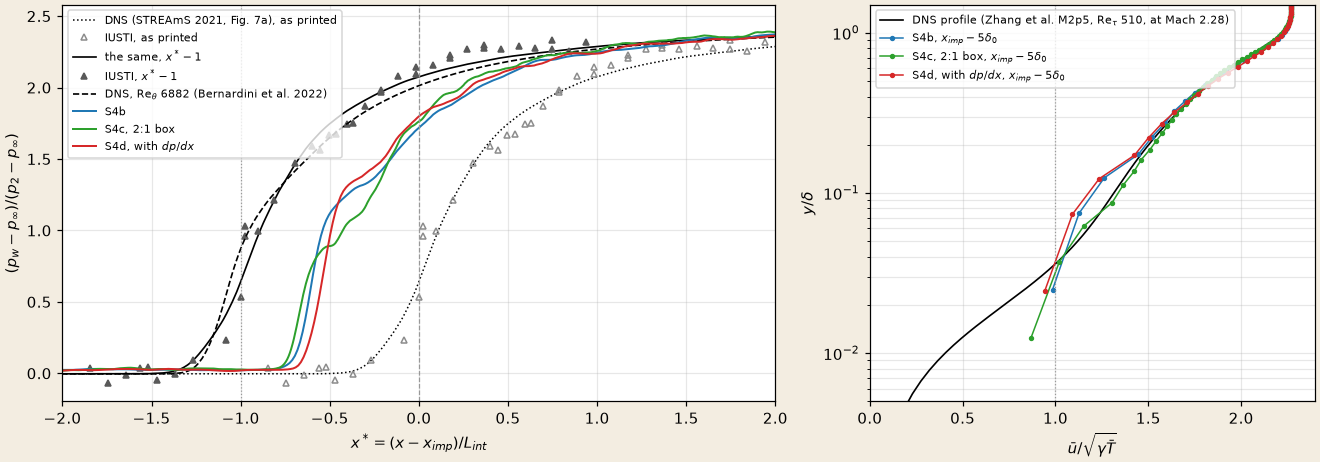
Left: the references as printed (dotted, open triangles) and shifted (solid, filled), the DNS at sbli_oracle.py fields and compression; make_doc_figures.py --only sbli-onset.
| S4b | S4c, 2:1 box | S4d, with | DNS, | |
|---|---|---|---|---|
| 3.16 | 3.05 | 3.13 | 3.30 | |
| wall pressure at 5 % of | ||||
| at 50 %: | ||||
| 0 | 0 | 0.60 | 2.16 ( | |
| incoming layer at |
fields, compression), 0.01 above compare's in the tables above.
- The incoming layer is not the cause. Its mean Mach number is the DNS profile's to 0.03 above
and to 0.15 at the 2nd cell ( , lower: the log-layer mismatch of the wall model), and its mean sonic height, – , is the DNS profile's . The first cell, below that height, runs at against the DNS's 0.85: the wall model's slip, one cell thick. - The compression is late by about
, – , on every grid and model. Below it crosses the layer as a vertical front at to ; above, it is the incident shock. The reflected shock's apparent origin is right ( within 5 %), the plateau behind the impingement too. - What is missing is the separation. In the DNS a bubble of
starting at lifts the flow and carries the compression to . The equilibrium model opens none (S4b, S4c) or a quarter of it (S4d), and the late compression follows. Halving the near-wall cells (S4c) leaves the onset where it was. The pressure-gradient term moved the onset by downstream. S4e qualifies this bullet and the first: without the model's eddy viscosity below the near-wall layer slows and the onset moves upstream with no bubble (below). - For the next wall model, non-equilibrium: the target is the DNS's bubble (
to ) and its wall pressure, half-way at . The run's wall pressure is printed by sbli_oracle.py compare(at fixed, against both DNS) and compression(where it reaches 5, 10 and 50 %); the oracle reports the run's, the DNS's is quoted from Bernardini et al. (2022).
Wall models for this interaction in the literature
Before a new wall model, what the literature says about wall-modelled LES of separating interactions, and the test it suggests on these runs.
| Source | Case | Finding |
|---|---|---|
| Hickel, Touber, Bodart & Larsson (2012, CTR Summer Program) | this interaction (IUSTI, | Above the viscous layer the convective term balances the pressure gradient (Bernoulli), so a model that keeps |
| Larsson, Kawai, Bodart & Bermejo-Moreno (2016, Mech. Eng. Rev. 3) | review | Equilibrium models can be accurate in these interactions "provided that the outer part of the boundary layer is well resolved" (a duct interaction near incipient separation; a ramp at |
| Fu, Karp, Bose, Moin & Urzay (2021, JFM) | Mach 6, laminar inflow, transitional interaction | The equilibrium-model LES delays the separation and advances the reattachment: a shorter bubble than the DNS's (the symptom here, in a different regime) |
| De Vanna, Bernardini, Picano & Benini (2022, IJHFF 98) | this interaction (IUSTI, | An equilibrium model coupled through a wall viscosity added to the molecular one, the no-slip condition kept: the first cell sets the sign of the wall stress, so |
Against these runs. S4b's grid (sbli_oracle.py apriori --ypg 4, the port of the pressure-gradient model with
| model, no | with | Bernoulli-consistent, | DNS, | |
|---|---|---|---|---|
| S4b: | 0 | 2.81 | 1.01 ( | 2.16 |
| S4c: | 0 | 2.54 | 1.53 ( |
- The a priori numbers bound the model, not the run. S4d's run kept a quarter of its a priori bubble (0.60 against 2.81), and its strongly negative
left the interaction where it was: the resolved flow above the matching height decides. A Bernoulli-consistent model alone is unlikely to reach . - The suspect is the resolved near-wall flow. The first cell runs at
– against the DNS profile's 0.85 at that height (above): extra momentum at the wall that the adverse gradient has to stop. The model's eddy viscosity below the matching height ( wall_model_eddy_viscosity) shapes that layer, so S4e takes it out.
Without the eddy viscosity below the matching height
| Setup | |
|---|---|
| start | S4b's last state ([amr] balance_static = .false.) |
| model | S4b's without wall_model_eddy_viscosity (the cells below |
| run | to sbli_oracle.py compare --t0 1300, fields, compression); the input is S4b's line of tbl_cases_s4.txt without --wm-eddy-viscosity, with --restart --time-max 1450 (no case file: a one-off restart) |
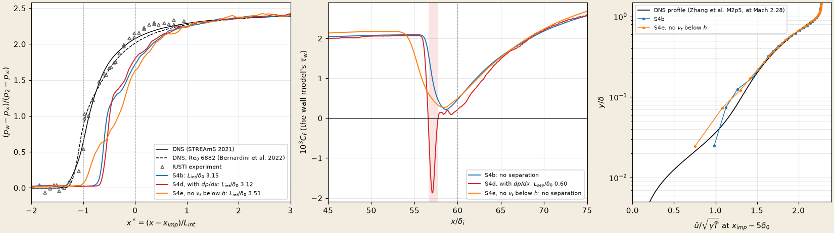
Left: the mean wall pressure of S4b, S4d and S4e against the DNS and the experiment; middle: make_doc_figures.py --only sbli-nonu.
| S4e, no eddy viscosity below | S4b | DNS, | |
|---|---|---|---|
| 3.51 | 3.16 | 3.30 | |
| wall pressure at 5 % of | |||
| the same at 50 % | |||
| separation: | 0, | 0, minimum | 2.16 |
| incoming layer at | 0.75 (DNS profile 0.82 there) | 0.98 (DNS profile 0.83) | |
| the same: second and third cells | 1.08, 1.30 (DNS 1.23, 1.37) | 1.13, 1.26 (DNS 1.24, 1.37) | |
| the same: sonic height | |||
| incoming layer: | 1.85, 0.572, 5463 | 1.81, 0.531, 5271 | |
- The eddy viscosity moves the onset, not the separation. Without it the first cell slows from
to 0.75, the sonic line rises from to , and the compression starts earlier: about two thirds of the way to the DNS at 5 % of the rise, 40 % of the way at 50 %. overshoots the DNS by 6 % (S4b undershoots by 4 %). The mean flow still does not separate, and the minimum of stays near S4b's. The pressure-gradient term (S4d) did the opposite: a bubble, the onset moved by downstream. - The incoming layer is not the DNS's either way. S4b's first cell is too fast and its next two too slow; S4e's first three are all too slow, and the sonic height goes from 15 % below the DNS's to 70 % above.
grows by 8 % and upstream by 5 %: S4e changes the layer that meets the shock, so it is a diagnostic, not a candidate setting. The run stayed stable for its 250 time units (the eddy viscosity was introduced against the first-cell drain of the Mach 3 channel, turbulence); longer runs were not made. - The mean is short. 150 time units against S4b's 890; the interim mean over
– gave , the full one 3.51. - What it points to. The two features have different levers: the onset answers to the momentum of the resolved near-wall layer, the separation to the sign of
. A Bernoulli-consistent model changes only (a priori – , above), so it is expected to open a bubble without moving the onset, as S4d did; the onset needs an incoming near-wall layer closer to the DNS profile, which is the matching between the model and the resolved cells, not the model's momentum balance.
The near-wall cells of the incoming layer
Before changing how the model meets the resolved cells: how far the cells of the incoming layer are from the DNS profile the inflow is made from, on both grids and with and without the eddy viscosity below
| Setup | |
|---|---|
| data | the span and time averages of sbli_oracle.py fields at |
| reference | reference/tbl_m2p28_profile.txt at the cell centres, |
| figure | make_doc_figures.py --only sbli-cells |
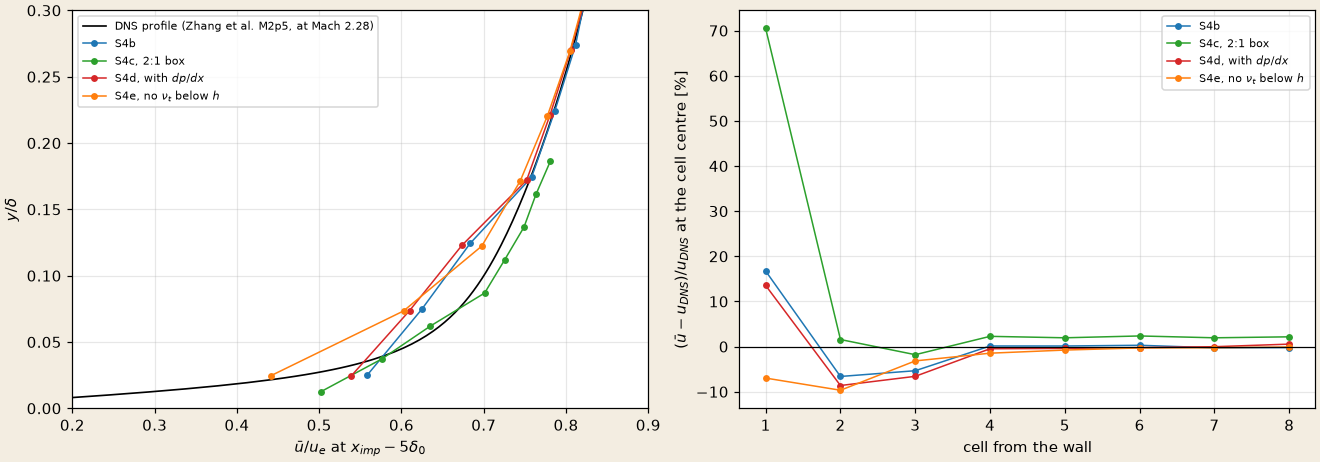
Left: the mean velocity of the first 8 cells of S4b, S4c, S4d and S4e against the DNS profile; right: the difference of each cell from the DNS at its centre. A cell holds the mean over its height: in the first cell, where the profile bends, the DNS's cell mean is below its centre value, so the excess of the runs is a lower bound.
| 1 | 2 | 3 | 4 | |
|---|---|---|---|---|
| DNS at S4b's centres ( | 0.478 | 0.669 | 0.722 | 0.757 |
| S4b | 0.558 (+17 %) | 0.625 ( | 0.684 ( | 0.758 (0 %) |
| S4d, with | +14 % | 0 % | ||
| S4e, no eddy viscosity below | 0.441 ( | 0.602 ( | 0.698 ( | |
| S4c, the box ( | +70 % | +2 % | +2 % |
The mean stress through the face between cells 1 and 2, in units of
| viscous | resolved | the model's eddy viscosity | sum | |
|---|---|---|---|---|
| S4b | 0.03 | 0.20 | 0.59 | 0.82 |
| S4e | 0.08 | 0.33 | — | 0.41 |
- The first cell slips with the eddy viscosity and lags without it. With the model's eddy viscosity below
it is 14–17 % faster than the DNS on S4b's grid and 70 % on S4c's finer one; without it 7 % slower. - Cells 2 and 3 are 5–10 % slow on S4b's grid, within 2 % on S4c's. That is the log-layer mismatch of a coarse near-wall grid (Kawai & Larsson 2012), and S4c's
removes it. From the 4th cell up every run is within 2.5 % of the DNS. - The budget does not close on the means. No subgrid model runs (the hybrid KEP-WENO scheme is the implicit LES), so with the eddy viscosity the explicit stresses carry 0.82 of
through the first face, without it 0.41. The rest is the scheme's dissipation, or the correlation of the eddy viscosity with the strain, which the means cannot separate: whether the resolved and the modelled stress overlap below is not measurable from these fields. - A DNS-like incoming layer does not move the onset. S4c's layer is the DNS's from the second cell up, and its onset is S4b's (above). S4e moves the onset with a layer slower than the DNS's. So matching the model to the resolved cells better, by itself, is not the lever for the interaction. The DNS's onset comes with its bubble, and the separation is what the runs lack (S4d opened a quarter of it, above).
The pressure gradient without the convection, with it, and without the eddy viscosity
Two more restarts of S4b at sbli_oracle.py compare --t0 1300, fields, compression), as S4d and S4e:
| Setup | S4g | S4f |
|---|---|---|
| model | S4d's (wall_model_pressure_gradient, filter 10) with wall_model_pressure_gradient_ypg = 4: the Bernoulli-consistent variant (turbulence) | S4d's, without wall_model_eddy_viscosity |
| question | does the consistent model keep a bubble? (a priori | does S4d's bubble grow when the near-wall flow is slower (S4e's layer)? |
| run | one node (4 A30), 0.97 s per step (S4d 0.92, S4e 0.68), 24 checkpoints | one node (4 A30), 3 h 52 min, 22 checkpoints |
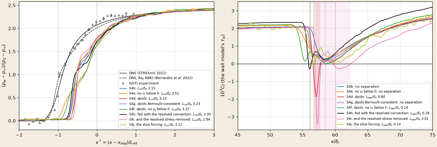
Left: the mean wall pressure of S4b, S4e, S4d, S4g, S4f, S4h (black, below) S4i (pink, below) and S4j (olive, below) against the DNS and the experiment; right: compare's, 0.01 below the table's. make_doc_figures.py --only sbli-pg-runs.
| S4b | S4e, no | S4d, | S4g, Bernoulli-consistent | S4f, | DNS, | |
|---|---|---|---|---|---|---|
| 3.16 | 3.51 | 3.13 | 3.24 | 3.37 | 3.30 | |
| 0 | 0 | 0.60 | 0 | 0.14 ( | 2.16 | |
| 0.21 | 0.27 | 0.15 | ||||
| 5 % of the rise, ahead of | ||||||
| 50 % of the rise | ||||||
| first-cell Mach number at | 0.98 | 0.75 | 0.94 | 0.95 | 0.70 | 0.83 |
- The consistent model does not separate. With convection balancing the pressure gradient above
(a few viscous lengths of the gradient, far below ), stays positive: S4g's dips to , S4b's 0.21, and its interaction is S4b's (onset within , within 0.08). S4d's bubble was the pressure gradient acting over the whole layer, the inconsistency Hickel et al. (2012) point out; a priori the consistent model kept of it, the run none. - A slower near-wall flow does not grow S4d's bubble. Without the eddy viscosity (S4f) the first cell slows to
, as in S4e, and the bubble shrinks from 0.60 to and moves downstream, toward the impingement ( –58.6 against S4d's 56.6–57.7); its also dips to at , where its compression starts, without reversing; the onset moves upstream as in S4e, by a little less ( against 3.55 at 5 %). The two levers do not add: each moves its own feature, and together they move both less. - What none of the five runs does. The DNS separates over
from ; the runs open at most and only with the inconsistent model. The sample sits at and about ten times lower ( under the interaction's gradient); where the reversed layer is thinner than the sample still moves downstream, and an equilibrium-type model, which takes from that sample and a consistently balanced gradient, cannot see the reversal. The DNS's bubble is taller than in its large state, and the runs' own mean reversed layer lies below (below). The convection the reversal needs is the flow's own, which a model fed with the resolved field (the integral model of Yang et al. 2015, the thin-boundary-layer equations with convection) carries and these do not.
The reversed flow: the DNS's bubble and the runs' below the sample
Whether a reversed layer can hide below the matching height: how tall the DNS's bubble is, and where the runs' own reversed flow sits.
The DNS. Bernardini et al. (2022) give the bubble's length (
The runs. sbli_oracle.py reversal reads each checkpoint in
| S4b | S4c, 2:1 box | S4d, | S4e, no | S4f, | S4g, Bernoulli-consistent | |
|---|---|---|---|---|---|---|
| checkpoints | 71 | 21 | 24 | 23 | 22 | 24 |
| area with | 0.068 (0.142) | 0.069 (0.084) | 0.049 (0.086) | 0.140 (0.200) | 0.113 (0.191) | 0.077 (0.106) |
| highest reversed cell of a column, 99th percentile, mean (max), | 0.31 (0.44) | 0.30 (0.40) | 0.31 (0.44) | 0.38 (0.52) | 0.38 (0.52) | 0.34 (0.49) |
| first cells reversed | 9.5 % | 14.5 % | 6.1 % | 23.3 % | 17.9 % | 9.8 % |
| third cells (the sample) reversed | 5.1 % | 8.7 % | 3.9 % | 8.2 % | 6.6 % | 5.9 % |
| time-mean | none | none | none | |||
| time-mean | none | cell 2 | none | none | none | none |
compare) | 0 | 0 | 0.60 | 0 | 0.14 | 0 |
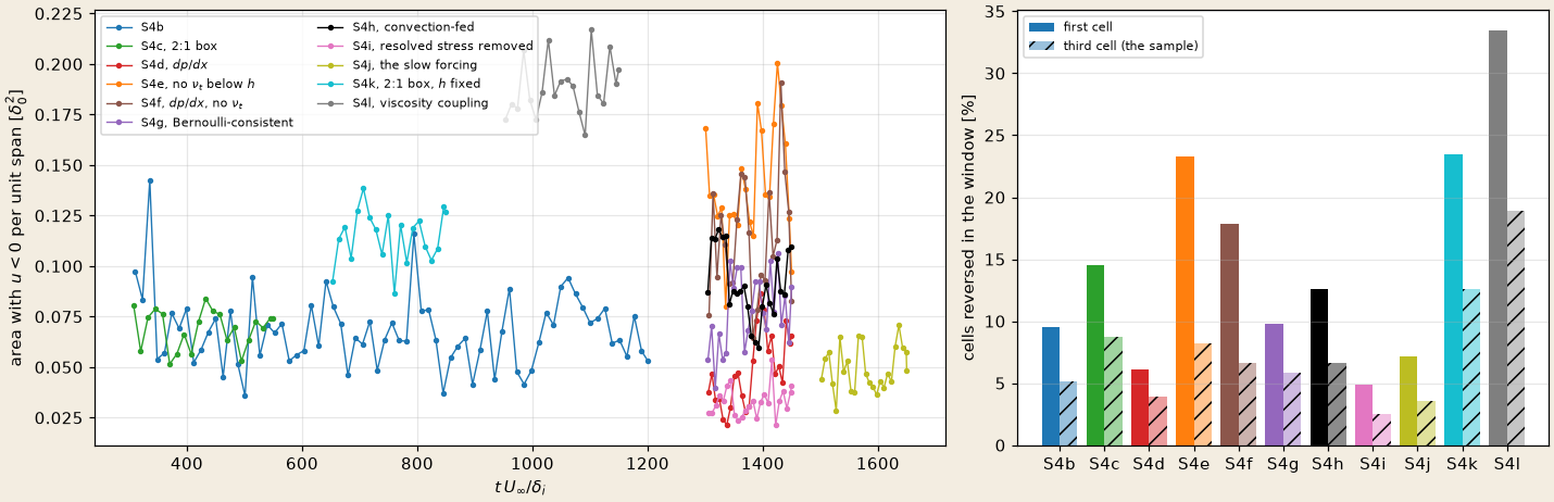
Left: the area with sbli_oracle.py reversal, make_doc_figures.py --only sbli-reversal. The time-mean reversal of the cells is printed by sbli_oracle.py compression.
- The runs reverse as high as the DNS's large state, but rarely. In every run some columns reverse up to
– ; the span-averaged area stays at 0.02– , within about twice its mean in each run (S4b's 71 checkpoints: 0.04–0.14 around 0.068), where the DNS's bubble area has a bimodal distribution with a long tail of large excursions (their Fig. 9; its normalisation is not given, and a single slice is not a span average, so the areas themselves are not compared). The sample sees these reversals: its cell is reversed 35–64 % as often as the first cell. - In the mean, three runs separate below the sample. S4c's resolved flow reverses in the mean over
in its first cell and in its second; S4e's over ( to , against the DNS's to ), S4f's over ; the third cell, the sample, never. The wall model's , which takes the sample, stays positive there: comparereports no separation for S4c and S4e, andfor S4f. - Under that layer the wall stress has the wrong sign. A positive
takes streamwise momentum out of a first cell whose mean flow is already reversed, where the wall would push it forward. The model is consistent only while the reversed layer reaches . - So the bubble is partly there, and the oracle's
misses it. The mean reversal of the first cell is the separation a wall-resolved run would report; on it, S4e is at half the DNS's length and the onset of its reversal is at , against . What the equilibrium-type models lack is a wall stress consistent with a reversed layer below : a model fed with the flow's own convection between the wall and (thin-boundary-layer equations, an integral model) has it by construction.
A priori: the wall model fed with the resolved convection
The thin-boundary-layer balance between the wall and sbli_oracle.py convective):
| equilibrium | Bernoulli-consistent (S4g's) | fed with the resolved convection | mean | ||
|---|---|---|---|---|---|
| S4b's mean field | 0 | 2.86 | 1.01 | 3.04 ( | none |
| S4d's | 0 | 2.88 | 0.74 | 2.79 | none |
| S4e's | 0 | 2.57 | 1.31 | 3.33 ( | 1.08 |
| S4f's | 0 | 3.11 | 1.31 | 2.98 | 0.72 |
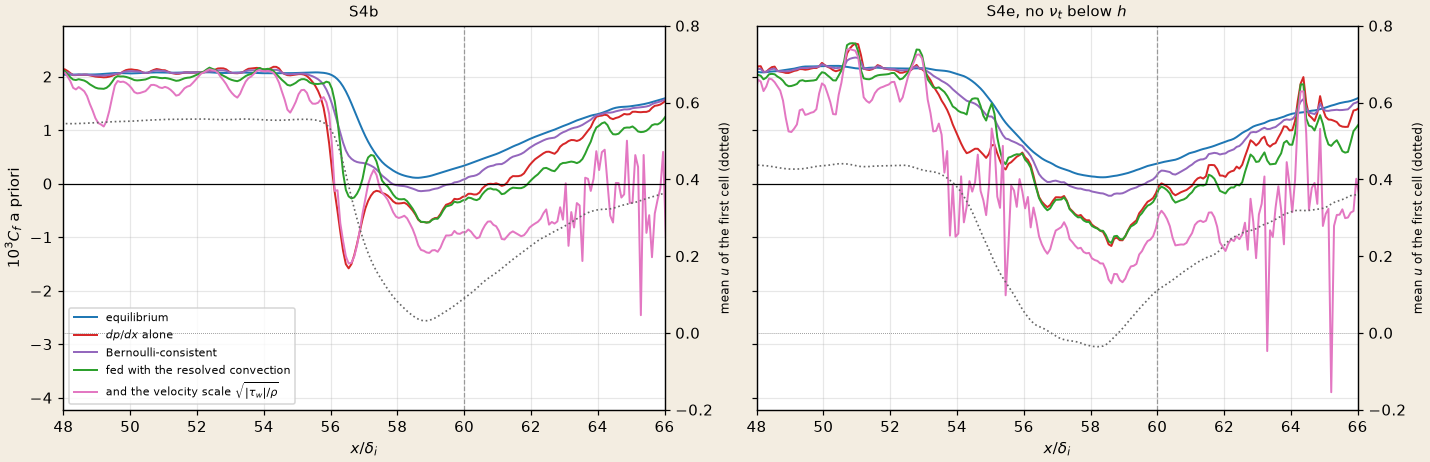
sbli_oracle.py convective, make_doc_figures.py --only sbli-convective.
- Where the resolved flow obeys Bernoulli, the model follows it. At the steepest gradient (
) the resolved convection of cells 1–6 balances 0.9–1.4 of , and the model fed with it loses the spike of the pressure gradient alone ( there for S4b), as the Bernoulli-consistent model does. - Where the resolved near-wall flow is slow or reversed, the convection is small (0 to 0.3 of
in cells 1–3 over –58.5) and the model behaves as the pressure gradient alone: over about , from , downstream into the reattachment. - The a priori does not tell this model from S4d's (2.8–3.3 against 2.6–3.1), and S4d's run kept a fifth of its a priori bubble. Unlike S4d's model, this one changes with the resolved flow: its
turns negative where the resolved convection stops balancing the pressure gradient, which is where S4c, S4e and S4f reverse below . Only a run says whether the feedback opens the DNS's bubble.
The run: S4h
S4b restarted at wall_model_pressure_gradient, filter 10, wall_model_convection; turbulence), the eddy viscosity below
| S4h, fed with the resolved convection | S4d, | S4g, Bernoulli-consistent | S4b | DNS, | |
|---|---|---|---|---|---|
| 3.36 | 3.13 | 3.24 | 3.16 | 3.30 | |
| 0.18 ( | 0.60 ( | 0 | 0 | 2.16 ( | |
| 0.15 | 0.21 | ||||
| time-mean | none | none | none | ||
| 5 % of the rise, ahead of | |||||
| 50 % of the rise | |||||
| first-cell Mach number at | 0.91 | 0.94 | 0.95 | 0.98 | 0.83 |
reversed area per unit span, mean (reversal), | 0.091 | 0.049 | 0.077 | 0.068 | |
| +5, +6, +9.5, +12 % | +1, +1, −2, −2 % | 0, 0, −3, −3 % |
- The interaction moves toward the DNS.
is the DNS's within 2 % (the closest of the runs), the onset moves upstream by at 5 % and at 50 % of the rise, the first cell slows from to 0.91 (the DNS profile 0.83), and the wall stress reverses at , where the DNS's bubble begins. The bubble is short, against ; the resolved first cell reverses in the mean over another further down. - The zero-gradient layer moves too, which it should not. Upstream of the interaction
rises by 5 % near the inflow and by 12 % ahead of the interaction, where S4d and S4g stay within 3 % (S4e and S4f, without the eddy viscosity, within 7 %), and the recovery behind the reattachment is higher still. The convection fed to the model is the instantaneous resolved one, and its time mean holds the gradient of the resolved shear stress, , large in the cells below (the budget above: 0.2 of through the first face, about 1 by the third). The model's own eddy viscosity already carries that stress: it is counted twice, and grows. Park & Moin (2014) meet the same double count in their thin-boundary-layer model fed with the LES and reduce the model's eddy viscosity dynamically, so that modelled and resolved stresses at add up to the total. - So the convection is a lever, and this form of it is not yet a model. It moves both the onset and
the right way, which no equilibrium-type variant did, but a model that changes the zero-gradient layer by 10 % fails the layer before the interaction. The correction is the reduced eddy viscosity (or the convection of the mean flow only), checked on the zero-gradient boundary layer before the interaction: S4i, below.
The run: S4i
S4h's model with wall_model_resolved_stress (turbulence): the filtered resolved shear stress of the convection cells removed from the forcing, and the eddy viscosity's velocity scale from
| S4i, the resolved stress removed, scale from | S4h, fed with the resolved convection | S4b | DNS, | |
|---|---|---|---|---|
| 2.94 | 3.36 | 3.16 | 3.30 | |
compare) | 0.18 | 0 | 2.16 ( | |
| 0.21 | ||||
| time-mean | none (its minimum | none | ||
| 5 % / 50 % of the rise, ahead of | 2.63 / 2.23 | 2.34 / 1.96 | 4.13 / 3.60 | |
| first-cell Mach number at | 0.98 | 0.91 | 0.98 | 0.83 |
| reversed area per unit span, mean (max), | 0.033 (0.054) | 0.091 | 0.068 (0.142) | |
| first / third cells reversed | 4.8 % / 2.5 % | 9.5 % / 5.1 % | ||
| +5, +6, +9.5, +12 % | ||||
A priori on the mean fields (convective), | convection-fed, scale | and the scale | |
|---|---|---|---|
| S4b's mean field | 56 % | 54 % (min | 81 % (min |
| S4e's | 52 % | 66 % (min | 94 % (min |
| S4i's | 42 % | 44 % (min | 66 % (min |
- The wall stress reverses, the flow does not.
is negative over two stretches, deep at the foot of the compression ( –57.79, down to , S4d's inconsistent balance ) and shallow behind the impingement ( –62.4). Between them, at –59.7, it is positive: there the first cell is slowest ( ), while at the deep stretch it moves at 0.33. The resolved flow reverses less than in any earlier run (half S4b's area and first-cell fraction), and its first cell never reverses in the mean. - The interaction shrinks.
falls from 3.16 to and the compression starts later than S4b's (5 % of the rise ahead of , against 2.34; the DNS 4.13): the opposite of S4h's shift. A negative wall stress under a forward first cell pushes the near-wall flow downstream, against the pressure rise. - The cause is the velocity scale, and the mean fields show it a priori. With the scale from
, the eddy viscosity vanishes as approaches zero, the model's layer becomes laminar, and the integrated adverse forcing (of order ) outweighs (about ): jumps to the negative branch. On S4b's mean field the variant is negative over 81 % of the interaction (the scale with 54 %) with a minimum three times deeper, and its sign changes 23 times along , against 2 to 4 for the other variants. The a priori was run after S4i; it would have stopped the run. - So the zero-gradient gate is necessary, not sufficient. The scale that removes the zero-gradient bias (the forcing's fluctuation in
) also removes the eddy viscosity that the adverse gradient needs. Upstream the run confirms the zero-gradient result: within 6 % of S4b's (S4h's +5 to +12 %), lower behind the inflow, as in the gate's recovery stretch.
A priori: the velocity scale of the eddy viscosity
S4h's scale, sbli_oracle.py convective), and on the filtered averages of the Mach 2.5 zero-gradient layer kept in the .wmf of two runs (boundary layer, wmf_apriori.py), over the developed stretch
| Velocity scale, | layer | sign changes of | of them beyond | fastest first cell under |
|---|---|---|---|---|
| 4, 4, 6 | 4, 2, 4 | 0.76, 0.60, 0.80 | ||
| 23, 30, 22 | 17, 16, 16 | 0.93, 0.89, 0.99 | ||
| 17, 27, 24 | 11, 12, 16 | 0.90, 0.89, 1.01 | ||
| 10, 7, 10 | 2, 2, 4 | 0.66, 0.89, 0.74 | ||
| 4, 4, 6 | 4, 2, 4 | 0.76, 0.60, 0.80 | ||
| 4, 4, 6 | 4, 2, 4 | 0.76, 0.60, 0.80 | ||
| the same, | 4, 6, 4 | 4, 4, 4 | 0.86, 0.83, 0.87 | |
| 4, 4, 6 | 4, 2, 4 | 0.76, 0.60, 0.80 | ||
| 4, 4, 2 | 2, 2, 2 | 0.93, 0.40, 0.96 |
The slow forcing and gradient: on a mean field, its own (so on the mean fields the last row is the first, and the local stress the total stress of the slow forcing); on the layer, the mean over the stretch, the limit of a long time filter in a homogeneous layer. Two .wmf: the runs rs and rs2 of the boundary-layer gate.
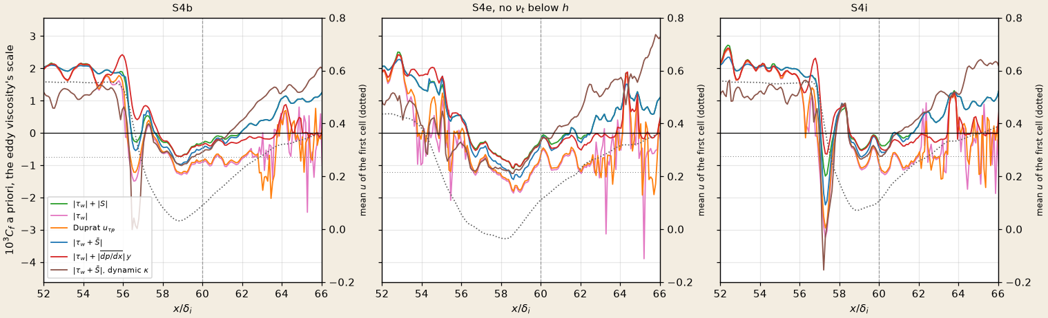
sbli_oracle.py convective, make_doc_figures.py --only sbli-scales.
- The mean forcing of the developed layer is its physical one. At the matching height the forcing with the resolved stress removed averages
(rs; in rs2) on , against a total-stress drop of in the DNS at the same (0.108); the of all the wall columns comes from the recovery behind the inflow ( , on ). - The bias is the fluctuating forcing inside the balance, not the scale alone. With the column's forcing every
-type scale lowers the layer's by 3 to 7 %, and in the scale raises it by 6 to 10 %; with the slow forcing in both the balance and the scale the layer is the equilibrium model's within 2 % (the only row that passes), and on the interaction it is S4h's , which does not chatter (4, 2, 4 sign changes beyond ) and keeps the eddy viscosity under the adverse gradient. Park & Moin's local stress with the column's forcing is close ( , %). - Duprat's scale is a near-wall scale. At the foot of the compression
– , against a forcing carried up to of : the eddy viscosity still vanishes with and chatters. - Matching
to the resolved slope at the third cell halves it (0.42–0.50 of 0.41 on the layer, 0.54–0.57 upstream of the interaction): the resolved velocity gradient there is too steep for the log law (the log-layer mismatch of wall-modelled LES), and the layer's falls by a third. The .wmfholds no fourth-cell averages, so on the layer the slope is one-sided, at. - The second interaction criterion is failed by nearly every model, the pressure gradient alone included (it passes on S4e's field only, where the first cell reverses): these mean fields come from runs whose near-wall flow does not slow, so a model forced by the measured pressure rise disagrees with them by construction. A priori, on another model's mean field, it cannot be met; only a run tests it.
- The a priori's absolute level is worth a few per cent. On the layer it puts S4i's scale at
to %, while its run (rs2) kept within 0.3 % of the equilibrium run over the same stretch: the sample is rebuilt from the averages (the speed of the third cell, the free-stream pressure, a fixed temperature), so differences between the rows are firmer than each row against the 2 % criterion.
The run: S4j
The slow-forcing model the a priori above favoured, after its zero-gradient gate (boundary layer: the forcing filtered over 100 keeps the layer within 1.9 % of the equilibrium model's, over 50 within 2.2 %): wall_model_resolved_stress, wall_model_velocity_scale = sum and wall_model_pressure_gradient_filter = 100. S4b restarted at
| S4j, the slow forcing | S4h, fed with the resolved convection | S4i, scale from | S4b | DNS, | |
|---|---|---|---|---|---|
| 3.12 | 3.36 | 2.94 | 3.16 | 3.30 | |
| 0.14 ( | 0.18 ( | 3.01, under a forward first cell | 0 | 2.16 ( | |
| 0.21 | |||||
| time-mean | none | none | none | ||
| 5 % / 50 % of the rise, ahead of | 2.09 / | 2.63 / 2.23 | 1.85 / 1.59 | 2.34 / 1.96 | 4.13 / 3.60 |
| first-cell Mach number at | 0.96 | 0.91 | 0.98 | 0.98 | 0.83 |
| reversed area per unit span, mean (max), | 0.049 (0.071) | 0.091 | 0.033 (0.054) | 0.068 (0.142) | |
| first / third cells reversed | 7.1 % / 3.5 % | 4.8 % / 2.5 % | 9.5 % / 5.1 % | ||
| +5, +6, +9.5, +12 % | |||||
| +30, +24 % |
- The incoming layer is S4b's. Upstream
stays within 2 % of S4b's, as the zero-gradient gate promised, where S4h's rose by up to 12 % and S4i's fell by 6 %. - The interaction is S4b's too.
is S4b's within 1.3 %, the compression starts later than S4b's, the first cell is as fast (Mach 0.96) and reverses less (7 % of the cells against 9.5 %). The wall stress dips to zero where the DNS's bubble begins, as S4h's did, over ; the resolved first cell does not reverse in the mean. - So S4h's gains do not survive the consistent model. S4h moved the onset
upstream and to the DNS's, but with a forcing filtered over 10 time units, which follows the interaction's unsteadiness, and a zero-gradient layer 5 to 12 % too high; filtered over 100, about half the low-frequency period ( , about 180 time units), the forcing is close to the mean, the zero-gradient layer is right, and the interaction returns to the equilibrium model's. Whether S4h's gain came from its response to the moving shock foot or from the bias of its incoming layer is not separated by these runs (a hypothesis).
Where the wall-modelled interaction stands
The S4 wall-model line is closed (#121). Eleven runs after S4b changed one thing each: the grid near the wall, the model's balance, its eddy viscosity, its matching height, its coupling to the face. The criterion throughout: consistent on the zero-gradient layer (its
| run | what changed against S4b | 5 % of the rise ahead of | incoming | ||
|---|---|---|---|---|---|
| S4b | the equilibrium model, | 3.15 | 0 | ||
| S4c | a 2:1 box at the wall, | 3.04 | 0 | 2.33 | +10.9 % |
| S4d | the pressure gradient in the model | 3.12 | 0.60 | 2.12 | |
| S4e | no eddy viscosity below | 3.51 | 0 | 3.55 | +4.8 % |
| S4f | S4d without the eddy viscosity below | 3.37 | 0.14 | 3.07 | |
| S4g | the Bernoulli-consistent pressure gradient | 3.24 | 0 | 2.44 | |
| S4h | fed with the resolved convection | 3.36 | 0.18 | 2.63 | +5 to +12 % |
| S4i | and the resolved stress removed | 2.94 | 3.01, under a forward first cell | 1.85 | |
| S4j | the slow forcing | 3.12 | 0.14 | 2.09 | within 2 % |
| S4k | S4c's box, | 3.26 | 0 (first cell reversed over 1.10) | 2.58 | +1.7 % |
| S4l | S4k with the viscosity coupling | 3.64 | 1.66 | 3.48 | +3.3 % (the flat plate |
| DNS, | 3.30 | 2.16 | 4.13 |
The incoming
- No variant passes both. Those consistent on the zero-gradient layer (S4d, S4j, S4k) keep the compression at least
behind the DNS's, and their wall stress separates over at most , S4d's by an inconsistent balance (the Bernoulli-consistent S4g has none). Those that move the onset or the bubble toward the DNS (S4e, S4h, S4l) shift the zero-gradient layer by 3 to 12 % (S4l by % on the flat plate), or reverse the stress under a forward flow (S4i). - The interaction length is within 10 % of the DNS's in every run but S4i (10.9 % short) and S4l (10.3 % long, the longest bubble); the separation and the onset are not reproduced by any.
- Where the gap is. The runs' reversed flow lies below the wall model's sample, in the first two or three cells (above); a model that sees only the sample keeps a forward stress over it (S4k), and coupling the stress to the first cell (S4l) makes it separate but slows the near-wall cells of the zero-gradient layer too.
- Not taken: a hybrid RANS/LES near the wall (#127); the viscosity coupling without the lower bound on the wall's subgrid viscosity (#126); a wall-resolved grid over the interaction.
Not done
- A separation of the right length and place, and the onset: no wall model tried here gives them with the zero-gradient layer kept (where the interaction stands); the S4 wall-model line is closed. The routes left: a hybrid RANS/LES near the wall (#127), a wall-resolved grid over the interaction.
- The late compression (
half-way against the DNS's ), unchanged by the near-wall grid and by the pressure-gradient term; moved 40 % of the way by taking out the eddy viscosity below (S4e), which also moves the incoming layer off the DNS's: the matching between the model and the resolved near-wall cells. - The wall-pressure fluctuations and the low-frequency unsteadiness.
- The recycling–rescaling inflow (S5).