7. Curves in 2-D

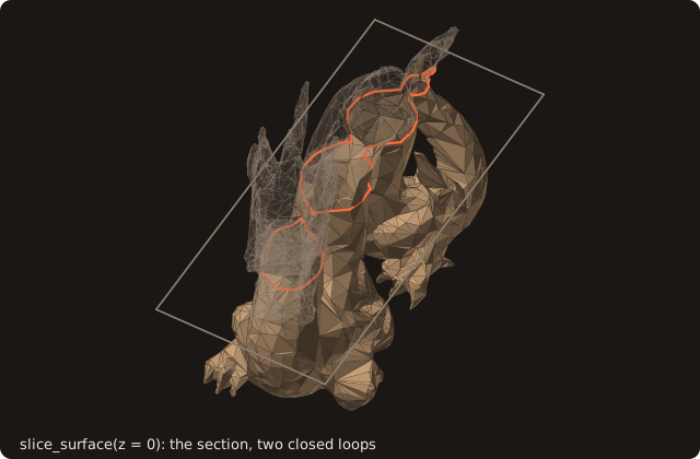
A 2-D run of the same case needs the body as a curve in a plane, not as triangles. slice_surface cuts the dragon by the plane z = 0, and the section is a curve_object with the same queries as a surface, in two dimensions.

use fossil, only : surface_stl_object, curve_object, distance_field_object, slice_surface, CURVE_VALID, STATUS_OK
use penf,   only : I4P, R8P

implicit none
type(surface_stl_object)    :: surface
type(curve_object)          :: section
type(distance_field_object) :: field
real(R8P)                   :: x(81), cp(2), d
integer(I4P)                :: i, open_loops, segment, vertex, status, crossings
integer(I4P), allocatable   :: pairs(:,:)

call surface%load_from_file(file_name='dragon-placed.stl', guess_format=.true.)
call slice_surface(surface, 3_I4P, 0._R8P, section, merge_collinear=.true., open_loops=open_loops, status=status)
print '(A,I0,A,I0,A,I0,A)', 'section z=0: ', section%get_loops_number(), ' loops, ', section%get_vertices_number(), &
                            ' vertices, ', open_loops, ' open'
print '(A,F9.6,A,F9.6,A,L1)', 'area ', section%get_area(), '  perimeter ', section%get_perimeter(), &
                              '  valid ', section%check_validity() == CURVE_VALID
call section%self_intersections(pairs, crossings)
print '(A,I0)', 'self-intersecting segment pairs ', crossings
call section%save_into_file(file_name='dragon-section.dat')

• slice_surface(surface, normal_axis, level, curve) cuts by the plane normal to axis normal_axis (1, 2, 3) at coordinate level. The curve lives in that plane with in-plane coordinates (u, v), the other two axes in cyclic order: for normal_axis = 3 they are (x, y). The crossings are exact constructions, with no tolerance: a vertex on the plane counts as above it.
• merge_collinear=.true. drops vertices between collinear segments. open_loops counts the chains that did not close, as happens on a surface with holes; such a curve can be closed by repair(tolerance=).
• The solid is on the left of every segment: outer loops run counter-clockwise, holes clockwise. check_validity() returns CURVE_VALID or the first defect found (CURVE_OPEN_LOOP, CURVE_WRONG_ORIENTATION, ...). By default it does not look for crossings; check_validity(check_self_intersections=.true.) does (CURVE_SELF_INTERSECTING), and self_intersections(pairs, n) returns the pairs of segments that cross, touch or overlap, decided exactly. The section is valid and still crosses itself once, at a fold of the non-manifold dragon; the distance queries do not mind, the cut cells and the swept geometry do (chapter 11 shows how the swept-geometry residual detects it).
• get_area and get_perimeter are the 2-D metrics. save_into_file writes the ASCII loop format, one u v per line, read back by load_from_file. Chapters 10 and 11 read dragon-section.dat.
• A curve can also be built from arrays: adopt_loops(u=, v=, loop_sizes=).

call section%compute_distance(p=[0._R8P, 0._R8P], distance=d, closest_point=cp, closest_segment=segment, &
                              closest_vertex=vertex)
print '(A,F10.6,A,2F10.6,A,I0)', 'd(0,0) ', d, '  closest ', cp, '  segment ', segment

• Points are p = [u, v]. compute_distance returns the signed distance, negative inside. Unlike the surface queries, curve distances are signed and not squared by default (is_signed=.false. for the unsigned one). It comes with the closest point, closest_segment, and closest_vertex (0 when the closest point is inside a segment). distance(p) and is_point_inside(p) are the short forms, distance_many the batch.

x = [(-0.6_R8P + 0.015_R8P * i, i = 0, 80)]
call field%initialize(x=x, y=x)                                   ! no z: a 2-D field
call field%compute(curve=section, status=status)
print '(A,I0,A,I0)', '2-D field: band cells ', field%get_band_cells(), ', inside ', count(field%phi < 0._R8P)

• initialize(x=, y=) without z makes a 2-D field; compute(curve=) runs the same band, sign and sweep stages as in chapter 6.

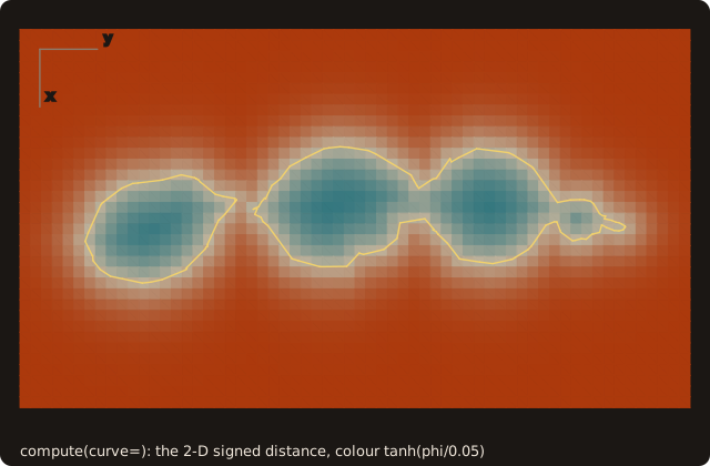
The colour saturates beyond about 0.1 from the wall; the field itself runs to the edges of the domain.

Running it

$ tut07_curves
section z=0: 2 loops, 152 vertices, 0 open
area  0.072609  perimeter  1.885961  valid T
self-intersecting segment pairs 1
d(0,0)  -0.015933  closest   0.015329 -0.004344  segment 20
2-D field: band cells 465, inside 327

The section has two closed loops, 152 vertices and an area of 0.072609. The origin is inside, 0.015933 from the wall. The 2-D field has 327 nodes inside on a spacing of 0.015, an area of 0.0736, against 0.0726 for the curve.

What you learned

slice_surface turns a surface into a curve_object; curves have the signed distance, the inside test and the distance field of surfaces, in (u, v) coordinates. Reference: 2-D geometry (curves), curve_object.

Next: 8. Immersed-boundary queries.