
Surface loads
What it does
A flow solver gets the force and the moment on a body from integrals over its wall. FOSSIL gives the geometry of those integrals, on the faceted wall itself: quadrature points on every facet (segment in 2-D) with their weights and normals, and probe points along the normal where the solver reads its flow. The solver evaluates the pressure p and the viscous traction τ at the samples; FOSSIL never interpolates the flow. With p and τ given, FOSSIL sums the force and the moment, per patch and per body too, the same bits on the CPU and on the device.
| Query | 3-D (surface_stl_object) | 2-D (curve_object) |
|---|---|---|
| Quadrature points, weights, normals, element, patch, body of every facet / segment | load_samples_3d(surface, samples=s) | load_samples_2d(curve, samples=s) |
| Probes along the normal: points, visibility, enclosing cells on the solver's lines | load_samples_3d(surface, x, y, z, s, lengths=) | load_samples_2d(curve, x, y, s, lengths=) |
| The body at a pose; the same on the device bit for bit, or left resident there | pose=, device=.true., resident=.true. | same |
| Several bodies at their poses: the samples of each in body order, probes visible against every body, the clearance to the nearest other body | load_samples_3d_bodies(surfaces, samples=s, poses=) | load_samples_2d_bodies(curves, samples=s, poses=) |
| Force, moment (2-D: its z component), per patch and per body, wetted area, from the solver's p and τ | integrate_loads(s, force, moment, pressure=, shear=) | same, a scalar moment |
| A wall field (per vertex or facet) at the closure's feet and ILW crossings, at the samples, at any point on a facet; values at the samples back to the vertices | transfer_to_closure, transfer_to_samples, transfer_field_3d, samples_to_vertices | the same generics, transfer_field_2d |
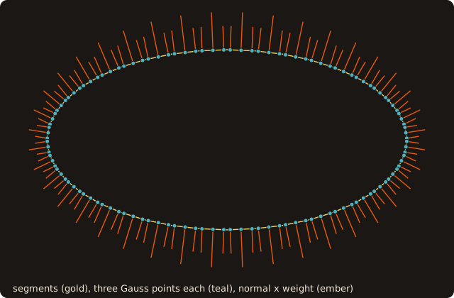
Three Gauss points per segment carry weights that sum to the segment's length; all of them sum to the perimeter. The figure program prints the counts of every figure on this page:
$ fig_ref_surface_loads
ellipse: segments 40, samples 120, sum of weights  1.9356982, perimeter  1.9356982
order 1: point  0.45000  0.30000  weight / area  1.000000
order 2: point  0.22500  0.15000  weight / area  0.333333
order 2: point  0.72500  0.15000  weight / area  0.333333
order 2: point  0.40000  0.60000  weight / area  0.333333
order 3: point  0.48378  0.09729  weight / area  0.223382
order 3: point  0.26418  0.40135  weight / area  0.223382
order 3: point  0.60203  0.40135  weight / area  0.223382
order 3: point  0.37747  0.73516  weight / area  0.109952
order 3: point  0.84890  0.08242  weight / area  0.109952
order 3: point  0.12363  0.08242  weight / area  0.109952
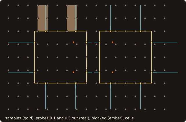
squares: samples 16, probes 32, blocked 4
sphere: facets 536, samples 1608, area  3.080745, 4 pi r^2  3.141593
force:  0.0000000  0.2502951  area 0.2502951  equal to 1e-14: T
Conventions
The samples follow three conventions, which the load integration (integrate_loads, below) keeps:
- L1, the integrand. The force on the body is F = ∫ (−p n + τ) dA over its wall, n the outward normal of the body, into the fluid; the moment about c is M = ∫ (x − c) × (−p n + τ) dA. τ is the viscous part of the wall traction (a 3-vector, a 2-vector in 2-D, per unit depth), supplied by the solver.
- L2, the quadrature. Each facet (segment) is integrated on its own plane by a rule of order 1, 2 or 3, with the facet's normal from its vertices, not the pseudo-normal: for the faceted wall the facet normal is exact. The weights include the facet area (segment length).
- L3, the flow. The solver evaluates p and τ. FOSSIL gives the probe points along the facet normal at the caller's signed lengths (+ into the fluid), whether each is visible from its sample, and its enclosing cell on the solver's lines (the low-side rule); no interpolation weights, as in the closure table.
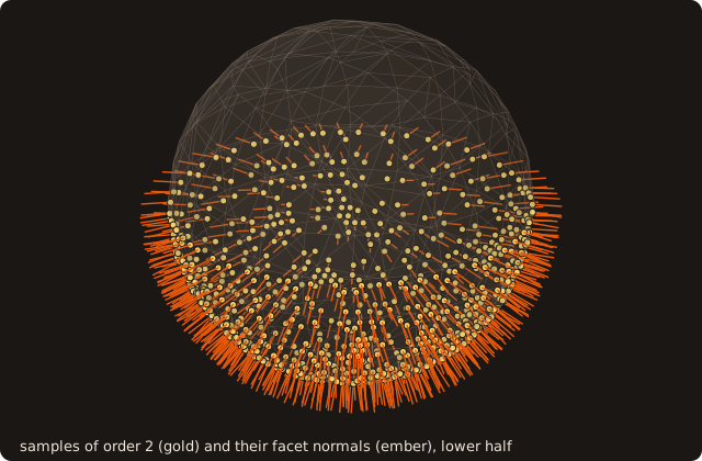
The normal is (v2 − v1) × (v3 − v1) / |…| of the facet's vertices: the vertex winding, outward on a surface that sanitize has oriented. In 2-D it is (dv, −du) / |…| of the segment i → next(i), the solid on its left: away from the centre on an outer loop, towards it on a hole.
The rules
| Order | 3-D points (barycentric) | 3-D exact to degree | 2-D points (on [0, 1]) | 2-D exact to degree |
|---|---|---|---|---|
| 1 | the centroid | 1 | 1/2 | 1 |
| 2 | (2/3, 1/6, 1/6) and its permutations, weights 1/3 | 2 | 1/2 ∓ √3/6 (Gauss–Legendre) | 3 |
| 3 | Dunavant's 6 points (a, a, 1 − 2a) for two values of a | 4 | 1/2, 1/2 ∓ √15/10 | 5 |

- The order-3 rule is the 6-point rule of Dunavant (1985), exact for degree 4 with positive weights and interior points (the 4-point rule of degree 3 has a negative weight); its constants are solved to 40 digits from the moment equations, then rounded.
- The weight of a sample is the rule's weight times the facet area (segment length), so the weights of a facet sum to its area to round-off. The samples of element e are s = (e − 1) q + 1 … e q, q =
samples%q(1, 3, 6 in 3-D; 1, 2, 3 in 2-D;load_rule_size(order, dims)). - A degenerate element (zero area or length; in 2-D also the missing segment at the end of an open polyline) gets zero weights and a zero normal; its probes sit at the sample and are not visible.
- A pressure linear in x is integrated exactly by every order (the centroid rule is exact for degree 1 on a flat facet): the buoyancy force of a closed body comes out to round-off. Its moment has a quadratic integrand, (x − c) p, exact from order 2 (below).
Probes, visibility and cells
With lengths(m) each sample gets m probes probe(:, k, s) = points(:, s) + lengths(k) normal(:, s): absolute, signed lengths (+ into the fluid), the same for every sample; a zero length gives the sample point itself.
- Visibility (
visible(k, s)): the open segment from the sample to the probe crosses no element. The kernels are those ofprobe_many(fossil_segment_visibility): in 3-D the exact ray–facet crossings, a crossing counted above 10⁻⁹ of the surface's box diagonal (the sample's own facet, crossed at 0, is ignored); in 2-D the exact segment test, the sample's own segment excluded. The probes need the SAH BVH (the default tree): on an octree surface they are refused. - Cells (
probe_cell(a, k, s)), when the solver's lines x, y[, z] are given: the low-side rule, x(i) < p ≤ x(i+1) gives i, outside the lines (or on the first one) 0, as in the closure table. Without the lines the samples have no cells (with_cells = .false.). - A probe into the solid (a negative length) is allowed; it is blocked as soon as it crosses the opposite wall.
How a solver fills p and tau
The solver evaluates p and τ at the samples, by its own means: at the wall from its closure, or from the flow at the probes (an image line, a wall model), interpolated in the cells FOSSIL gives. The force is then a sum over the samples, which integrate_loads does for it (below); written out:
force = 0._R8P
do s = 1, ls%n
   force = force + (-p(s) * ls%normal(:, s) + tau(:, s)) * ls%weight(s)
enddo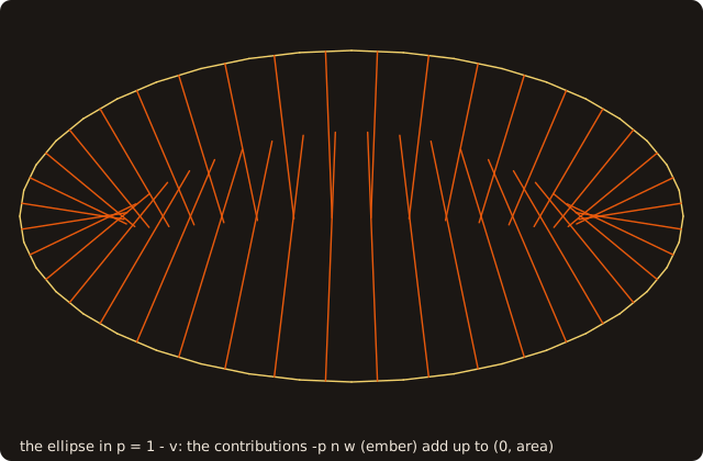
In p = 1 − v the force is the buoyancy, (0, area) per unit depth: one sample per segment gives it to round-off (the last line of the figure program's output). The weights and normals are the facet's, so the sum is the integral over the faceted wall; how close it is to the smooth body's depends on the facets, not on the rule.
Forces and moments
integrate_loads(samples, force, moment, pressure=p, shear=tau) sums the loads of the samples with the solver's pressure p(n) and viscous traction τ(d, n) at the samples (either or both):
- The integrand (L1). Each sample contributes f = w (−p n + τ), n the outward normal, into the fluid; its moment about c (
about, default the origin) is (x − c) × f. The force on the body is F = Σ f, the moment M = Σ (x − c) × f. In 2-D both are per unit depth and the moment is its component along the plane's normal axis, a scalar r_u f_v − r_v f_u. - The sums (L4). Compensated (Neumaier) sums in sample order, so in facet (segment) order: deterministic, and their error is that of the terms, not of their number. The same sums per patch (
per_patch_force,per_patch_moment) and per body (per_body_force,per_body_moment), sized by the largest patch and body ids of the samples; the wetted area (2-D length) Σ w asarea.
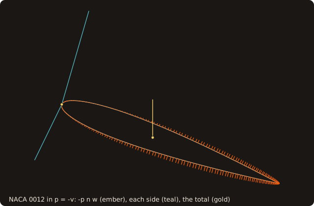
The two sides of the airfoil are two patches; their forces add up to the buoyancy (0, A), A the enclosed area, and their moments about the leading edge to that of the buoyancy at the centroid, A (x_c − c) × (0, 1):
$ fig_ref_surface_loads_forces
NACA 0012 at 20 degrees: segments 120, samples 240, area A  0.081669
force on the upper side -0.058489 -0.119863, lower side  0.058489  0.201531, total  0.000000  0.081669
moment about c: upper -0.097632, lower  0.129708, total  0.032076
buoyancy A =   0.081669, A (x_c - c) x (0, 1) =   0.032076;  equal to 1e-14: T
The exactness check: buoyancy. In a linear pressure p = p0 + g · x with τ = 0 the divergence theorem gives, on any closed faceted body of volume V (2-D: area A) and centroid x_c,
F = −g V, M = V (x_c − c) × (−g).
The force's integrand p n is linear on a flat facet, integrated exactly by every rule; the moment's, (x − c) p, is quadratic, integrated exactly from order 2 (the centroid rule misses it: 5·10⁻³ of the moment on an irregular tetrahedron, nothing on a body symmetric enough to cancel it). The tests fossil_test_integrate_loads_3d and _2d check both identities on cube-01, an icosphere at a pose, two boxes (per body too), an irregular tetrahedron, a 64-gon, a disc with a hole, a NACA 0012 polygon unposed and posed and two discs, against V and x_c from mass_properties: every component within ε times the sum of the absolute terms (Σ w |p| + V |g|, for the moment Σ w |p| |x − c| + V |g| |x_c − c|); the largest error measured is 0.34 of that bound.
Host and device. Each sample's contribution comes from one kernel (load_force_3d_oac, load_force_2d_oac), in a loop that runs on the device with device=.true.: the samples, p and τ are read on the device where they are mapped (resident samples, a pressure the solver mapped itself), else copied in. The contributions then come back and are summed on the host in sample order, by the same code for both paths, so the totals agree bit for bit (loads device vs serial mismatches in the benches). On the host path the host arrays are read: call update_host on resident samples first.
call load_samples_3d(sphere, samples=ls, order=2_I4P, pose=pose)  ! the samples of the body at its pose
p = 1._R8P - ls%points(3, :)                                      ! the solver's pressure at the samples
call integrate_loads(ls, force, moment, pressure=p, about=[0._R8P, 0._R8P, 0._R8P], area=area)
call sphere%mass_properties(volume=vol, center=xc) ; xc = to_world(pose, xc)
print '(A,3F11.7,A,F10.7,A)', 'force ', clean(force), '   buoyancy (0, 0, V), V =', vol, ' (faceted)'
print '(A,3F11.7,A,3F11.7)', 'moment', clean(moment), '   V x_c x (0, 0, 1) =', clean(vol * [xc(2), -xc(1), 0._R8P])
print '(A,F10.7,A,L1)', 'wetted area', area, ';  the identities to 1e-15: ', &
      max(maxval(abs(force - [0._R8P, 0._R8P, vol])), maxval(abs(moment - vol * [xc(2), -xc(1), 0._R8P]))) < 1.e-15_R8P
call sphere%enter_device
call load_samples_3d(sphere, samples=lr, order=2_I4P, pose=pose, resident=.true.)
call integrate_loads(lr, fd, md, pressure=p, about=[0._R8P, 0._R8P, 0._R8P], device=.true.)  ! read on the device
print '(A,L1)', 'device = host, bit for bit: ', all(transfer([fd, md], 0_I8P, 6) == transfer([force, moment], 0_I8P, 6))
call load_samples_reset(lr)
call sphere%exit_device
$ ref_surface_loads_forces
force 0.0000000 0.0000000 0.5187371 buoyancy (0, 0, V), V = 0.5187371 (faceted)
moment 0.1037474 -0.1556211 0.0000000 V x_c x (0, 0, 1) = 0.1037474 -0.1556211 0.0000000
wetted area 3.1262326; the identities to 1e-15: T
device = host, bit for bit: TThe cookbook integrates the pressure and a uniform shear on the unit cube.
Moving fields between the wall and the grid
A solver keeps fields on the wall, per vertex or per facet (a wall temperature, the displacement of a deforming wall), and needs their values where its closure and its loads look at the wall; and it computes fields at points of the wall (a wall stress at the load samples) that it wants back on the wall. fossil_field_transfer does both, on the geometry FOSSIL already has: every point carries the element it lies on.
- Wall to points (L5).
transfer_field_3d(surface, facets, points, values, vertex_field=): for points on (or projected onto) the facetsfacets(n), a per-vertex fieldvertex_field(ncomp, nv)(the vertices of the surface's vertex pool) interpolated with the barycentric weights (1 − s − t, s, t) of the point's closest point on its facet, the (s, t) oftriangle_closest_st, the solve of every distance query. A linear field is reproduced at any point of the facet to round-off; a point equal to a vertex takes that vertex's value bit for bit; a point off the facet takes the value of its closest point.facet_field=(ncomp, nf)instead: piecewise constant, copied.ncompcomponents: a scalar or a vector. An id outside 1..nf gives zeros. In 2-D,transfer_field_2d(curve, segments, points, values, vertex_field= | segment_field=)with (1 − s, s) of the clamped projection on the segment. - At the closure table and the load samples.
transfer_to_closure(surface, closure, values, vertex_field=, ilw_values=)reads the field at the feet (closure%element) and, withilw_values(ncomp, 2d, n), at the ILW crossings: the ghost's coordinates with the slot's axis set toilw_t, onilw_element; a slot without a crossing gives zeros.transfer_to_samples(surface, samples, values, vertex_field=)reads it at the load samples with the rule's own barycentric coordinates, the ones that placed them (no closest point, no pose). - Poses. With
pose=the points are in the world and the body at the pose, as in a posed closure table: each point is taken to the body frame (to_body) before its weights, so the field stays attached to the body's vertices. - Points to wall.
samples_to_vertices(surface, samples, values, field): values at the load samples to a per-vertex field, the direction a solver needs for a wall stress it computes at its samples (the wall-modelled setting of van Noordt et al. 2022). Per element, a linear fit of its q values in the barycentric coordinates (weighted least squares with the rule's weights; order 1: the constant;linear=.false.: the weighted mean), evaluated at each of its vertices; per vertex, the average of those values over its incident elements weighted by their areas (2-D lengths), in increasing element order with Neumaier sums. A smoothing projection, not an interpolation: a constant comes back exactly; values linear on every element (a field linear in space, on any mesh, or any vertex field brought to the samples bytransfer_to_samples) come back at every vertex to round-off from order 2; anything else is fitted per element and averaged over the vertex's ring, its noise smoothed with it.
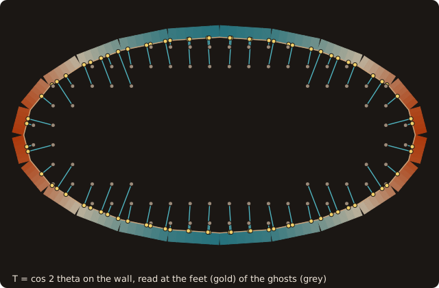
The figure's vertex field is cos 2θ at 24 vertices: linear along each segment, read at the feet of 80 ghost points. Back through the load samples, the same field returns unchanged (it is linear on every segment); cos 2θ evaluated at the samples themselves comes back to the vertices with the projection's error:
$ fig_ref_surface_loads_transfer
ellipse of 24 segments: 80 ghost points; T at their feet in -0.97253 ..  0.93885
linear field, vertices -> samples -> vertices, equal to 1e-14: T
cos 2 theta from the vertices (linear on each segment), the same round trip, unchanged to 1e-14: T
cos 2 theta at the samples, back to the vertices: largest error  0.02259 (a smoothing projection)
Host and device. Every value comes from one kernel per point (transfer_weights_3d_oac, transfer_weights_2d_oac, the rule kernels of the samples), per element and per vertex for the projection, in loops that run on the device with device=.true.: the inputs are read on the device where they are mapped (a resident closure table or load samples, a field the solver mapped itself), else copied in; the output is written on the device where the solver mapped it (then !$acc update host), else copied back. The per-vertex sums run one thread per vertex in its fixed order, so the two paths agree bit for bit (field transfer device vs serial mismatches in the benches; tests fossil_test_field_transfer_3d, _2d). The facet vertex ids (2-D the curve's vertices) are gathered on the host per call and copied in.
call fd_closure_3d(sphere, x + 0.3_R8P, x + 0.2_R8P, x + 0.1_R8P, [2_I4P, 2_I4P, 2_I4P], cl, pose=pose, ilw=.true.)
allocate(tf(1, cl%n), ti(1, 6, cl%n))
call transfer_to_closure(sphere, cl, tf, vertex_field=tw, ilw_values=ti, pose=pose) ! T at the feet, the crossingscall load_samples_3d(sphere, samples=ls, order=2_I4P, pose=pose) ! a wall stress known at the samples (world frame)
allocate(tau(2, ls%n), tv(2, pool%vertex_count()))
tau(1, :) = 0.1_R8P * (1._R8P + ls%points(1, :) - ls%points(3, :)) ! linear
tau(2, :) = 0.1_R8P * cos(4 * ls%points(3, :)) ! curved
call samples_to_vertices(sphere, ls, tau, tv) ! per vertex, area-weighted$ ref_surface_loads_transfer
ghosts 1808, ILW crossings 3792; T at the feet and crossings exact to 1e-12: T
vertices 1158; linear stress exact to 1e-14: T; curved stress, largest error 0.00086
device = host, bit for bit: Tcall transfer_field_3d(surface, facets, points, values [, status] [, vertex_field | facet_field] [, pose] [, device])
call transfer_field_2d(curve, segments, points, values [, status] [, vertex_field | segment_field] [, pose] [, device])
call transfer_to_closure(surface | curve, closure, values [, status] [, vertex_field | facet_field | segment_field]
[, ilw_values] [, pose] [, device])
call transfer_to_samples(surface | curve, samples, values [, status] [, vertex_field | facet_field | segment_field]
[, device])
call samples_to_vertices(surface | curve, samples, values, field [, status] [, linear] [, device])status = STATUS_INVALID_INPUT (a stderr message, the outputs zero) on no field or both, a size that differs, a table or samples of the other dimension (or not of this surface or curve), ilw_values from a table without ILW. The cookbook has the shortest program.
Several bodies
Two bodies in one flow share its probes: an image line out of one wall may enter the other body, and a wall that faces another across a narrow gap carries a load that depends on the gap. load_samples_3d_bodies(surfaces, x, y, z, samples) and load_samples_2d_bodies(curves, x, y, samples) sample an array of bodies, body b at poses(b), in one set:
- Each body as alone, in body order. The samples of body b are those
load_samples_3d(_2d) gives it at its pose, the same kernels, placed after those of bodies 1 … b − 1;elementis the facet (segment) of its own surface,bodythe index of the surface in the array,sub_bodythe element'sfacet_body(loop body). - Visibility is against every body. A probe is visible when the segment sample–probe crosses no element of its own body (as for one body) and no element of any other body, tested in that body's frame (the closure's test of several bodies).
- Clearance.
clearance(s)is the unsigned distance from the sample point to the nearest other body (second_body,second_foot: its closest point); huge without one. In a gap of width δ the facing samples have clearance δ: a lubrication or wall model reads it there; FOSSIL decides nothing. - Loads per body.
integrate_loadssumsper_body_forceandper_body_momentby the samples'body: the surfaces of the array here, thefacet_bodyshells of a single-body set.
| Field | Shape | Meaning |
|---|---|---|
body, sub_body | [n] | The body's index in the array; the element's facet_body |
clearance, second_body, second_foot | [n], [n], [d, n] | Distance from the sample point to the nearest other body, that body, its closest point |
with_bodies, bodies | scalars | A bodies set; the number of bodies |
A single-body set has these arrays with a zero last extent. With one body the bodies set equals the single-body set bit for bit in every other field (on a surface of one facet_body), and for bodies farther apart than the probes the samples of every body are its single-body set bit for bit (fossil_test_load_samples_bodies_3d, _2d).
$ fig_ref_surface_loads_bodies
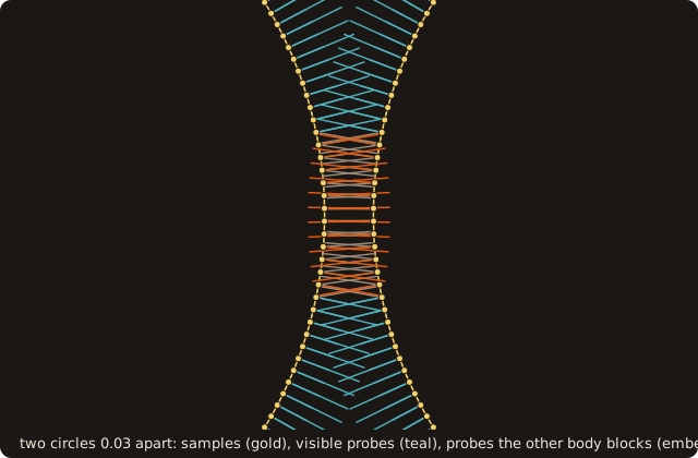
bodies: samples 400, probes blocked 24, within 2 h of the other body 28, least clearance 0.0301h = 0.02_R8P
poses = [pose_2d(0._R8P, [-0.265_R8P, 0._R8P]), pose_2d(0._R8P, [0.265_R8P, 0._R8P])] ! a gap of 0.03
call load_samples_2d_bodies(discs, samples=ls, poses=poses, lengths=[h, 2 * h]) ! order 2, two probes
print '(A,I0,A,I0,A,I0)', 'two discs: samples ', ls%n, ', of body 1 ', count(ls%body == 1), ', of body 2 ', &
count(ls%body == 2)
call load_samples_2d(discs(1), samples=alone, pose=poses(1), lengths=[h, 2 * h])
print '(A,I0,A,I0)', ' probes blocked: ', count(.not. ls%visible), ', disc 1 alone: ', count(.not. alone%visible)
print '(A,F7.4,A,I0,A,I0)', ' least clearance ', minval(ls%clearance), ', samples within 2 h of the other body ', &
count(ls%clearance < 2 * h), ', second body of sample 1: ', ls%second_body(1)
s = minloc(ls%clearance, 1) ! a sample of the gap
print '(A,2F8.4,A,I0,A,F7.4,A,2F8.4,A,2L2)', 'sample at', ls%points(:, s), ': body ', ls%body(s), ', clearance', &
ls%clearance(s), ' to', ls%second_foot(:, s), ', visible', ls%visible(:, s)
p = -ls%points(2, :) ! hydrostatic p = -v (rho g = 1, gravity -v)
call integrate_loads(ls, force2, moment2, pressure=p, per_body_force=fb, per_body_moment=mb)
print '(A,2F9.5,A,F9.5)', ' buoyancy per body (v)', fb(2, :), ', area of a disc', discs(1)%get_area()places(1) = pose_from_axis_angle([0._R8P, 0._R8P, 1._R8P], 0._R8P, [-0.55_R8P, 0._R8P, 0._R8P])
places(2) = pose_from_axis_angle([0._R8P, 0._R8P, 1._R8P], 0.4_R8P, [0.55_R8P, 0._R8P, 0._R8P]) ! 0.1 apart
call balls(1)%enter_device ; call balls(2)%enter_device ! map the array elements themselves
call load_samples_3d_bodies(balls, samples=ls, poses=places, lengths=[0.05_R8P, 0.15_R8P], device=.true.)
print '(A,I0,A,I0,A,F7.4)', 'two balls: samples ', ls%n, ', probes blocked ', count(.not. ls%visible), &
', least clearance ', minval(ls%clearance)
p = -ls%points(3, :) ! gravity -z
call integrate_loads(ls, force, moment, pressure=p, per_body_force=fb, device=.true.)
print '(A,F9.5,A,F9.5)', ' buoyancy of ball 2 (z)', fb(3, 2), ', its volume', balls(2)%get_volume()
call load_samples_3d_bodies(balls, samples=twin, poses=places, lengths=[0.05_R8P, 0.15_R8P])
print '(A,I0)', ' device path vs host path: mismatches ', load_samples_mismatches(ls, twin)
call balls(1)%exit_device ; call balls(2)%exit_device$ ref_surface_loads_bodies
two discs: samples 800, of body 1 400, of body 2 400
probes blocked: 44, disc 1 alone: 0
least clearance 0.0300, samples within 2 h of the other body 52, second body of sample 1: 2
sample at 0.0150 0.0017: body 2, clearance 0.0300 to -0.0150 0.0012, visible T F
buoyancy per body (v) 0.19632 0.19632, area of a disc 0.19632
two balls: samples 13872, probes blocked 175, least clearance 0.1018
buoyancy of ball 2 (z) 0.51874, its volume 0.51874
device path vs host path: mismatches 0- The two discs, 0.03 apart, have 400 samples each (order 2). Their 44 blocked probes are the ones that cross the gap; disc 1 alone blocks none (a convex body).
- The least clearance is the gap, 0.0300; the sample of least clearance sees its first probe (0.02, inside the gap) and not its second (0.04, across the other wall).
- The buoyancy of each disc in p = −v is its area (F = −∮ p n dA = A ∇v): each body's integral is exact for a linear pressure, whatever the other body.
- The balls are 0.1 apart: the least clearance is 0.1018 (the marching-cubes facets lie inside the sphere), and the device path returns the same samples.
The device path runs the single-body pipeline once per body into a work set, copies the sets into one, then per other body the clearance query (the sample points in that body's frame) and the visibility test: copies, comparisons and the shared query kernels, so host and device agree bit for bit (bench lines load samples bodies device vs serial mismatches). Map the array's elements themselves (call bodies(b)%enter_device): a copy of a mapped surface is not mapped.
Validation. The validation program fossil_val_bodies (about 4 s at -O2, 0.1 GB; its closure part is on the closure page) checks the samples of several bodies and the loads of each body through both paths.
- Locality. An icosphere and an ellipsoid (3-D, order 3, probes h and 2 h at h = 0.1), a NACA 0012 and an ellipse (2-D, h = 0.01), each at three pose pairs farther apart than the probes: the samples of every body are its single-body set at its pose, bit for bit, in body order (38 400 and 3 936 samples; 0 mismatches).
- Loads through the union. In p = p0 + g · x the force on each closed body is −g V_k and its moment V_k (x_c,k − c) × (−g), whatever the other body. FD:
load_samples_3d_bodies/_2d_bodies,integrate_loadswithper_body_force/per_body_moment, rule orders 1–3. FV:cut_cells_3d_bodies(walls=, piece_bodies=)/cut_cells_2d_bodies; the wall terms of body k are those withpiece_bodies%wall_body == k(the pressure and its gradient set to zero on the others), summed bycut_loads_3dwith the merged surface'scut_walls_gyration/cut_loads_2dwith the gradient. Largest errors per case, in units of ε times the sum of the absolute terms of the body (as above):
| Case | Wall terms (body 1, 2) | Contact terms per body | FV F | FV M | FD F (q = 1–3) | FD M (q = 2, 3) |
|---|---|---|---|---|---|---|
| two spheres, gap 0.25 h (h = 0.1) | 15 687, 15 693 | 0 | 0.23 | 0.28 | 0.23 | 0.28 |
| sphere + ellipsoid, gap ≥ 0.5 h | 15 687, 12 657 | 0 | 0.12 | 0.12 | 0.15 | 0.10 |
| unit cubes in face contact (aligned, shifted; h = 0.13, 0.125) | 678–816 | 113–136 | 0.03 | 0.03 | 0.06 | 0.09 |
| two circles, gap 0.25 h (h = 0.02) | 1 224, 1 224 | 0 | 0.23 | 0.11 | 0.23 | 0.11 |
| NACA 0012 + ellipse, gap ≥ 0.5 h | 1 024, 690 | 0 | 0.01 | 0.04 | 0.04 | 0.04 |
| unit squares in edge contact (aligned, shifted; h = 0.13, 0.125) | 32–36 | 8–9 | 0.06 | 0.07 | 0.12 | 0.07 |
- Every cut cell is trusted, contacts included. In a contact both bodies keep their wall terms on the contact face, with opposite vector areas, so each body's sum is the integral over its own closed surface: −g V_k. That is the identity, not the load in a flow: no fluid wets the contact, and a solver that imposes the contact force replaces the pressure on those terms (they lie on the contact plane; the program counts them).
Pass criteria (Are all tests passed? T iff all hold): 0 sample mismatches at every pose pair; per body the force within 1 (ε S_F) on both paths and every rule order, the moment within 1 (ε S_M) where it is exact (FD from order 2, FV with the gradient and the gyration); every cut cell trusted and every wall term labelled with a body; every call STATUS_OK.
Example
The ellipse at a pose on cell-centred lines, three Gauss points per segment and two probes; then a sphere, the samples left resident on the device.
h = 0.02_R8P
xc = [(-0.5_R8P + (i - 0.5_R8P) * h, i = 1, 50)] ; yc = [(-0.3_R8P + (j - 0.5_R8P) * h, j = 1, 30)]
pose = pose_2d(0.3_R8P, [0.05_R8P, 0._R8P])                       ! the body at its pose: turned, moved
call load_samples_2d(ellipse, xc, yc, samples, order=3_I4P, &     ! three Gauss points per segment
                     lengths=[h, 2 * h], pose=pose)               ! two probes along the normal, + into the fluid
print '(A,I0,A,I0,A,I0,A,F10.7)', 'ellipse: segments ', samples%ne, ', samples ', samples%n, ', visible probes ', &
      count(samples%visible), ', sum of weights ', sum(samples%weight)
print '(A,2F9.5,A,F9.6,A,2F9.5,A,I0)', 'sample 1: point', samples%points(:, 1), '  weight', samples%weight(1), &
      '  normal', samples%normal(:, 1), '  segment ', samples%element(1)
print '(A,2F9.5,A,2F9.5,A,2(2I3,:,","))', '  probes', samples%probe(:, 1, 1), ',', samples%probe(:, 2, 1), &
      '  cells', samples%probe_cell(:, :, 1)
call ellipse%enter_device
call load_samples_2d(ellipse, xc, yc, twin, order=3_I4P, lengths=[h, 2 * h], pose=pose, device=.true.)
print '(A,I0)', 'device path vs host path: mismatches ', load_samples_mismatches(samples, twin)
call ellipse%exit_devicecall sphere%enter_device ! the surface on the device, once
call load_samples_3d(sphere, xn, xn, xn, samples, order=3_I4P, lengths=[0.05_R8P, 0.1_R8P], &
resident=.true.) ! the samples stay on the device
print '(A,I0,A,I0,A,L1)', 'sphere: facets ', samples%ne, ', samples ', samples%n, ', resident ', samples%on_device
call samples%update_host ! (a device solver would read them there)
call load_samples_3d(sphere, xn, xn, xn, twin, order=3_I4P, lengths=[0.05_R8P, 0.1_R8P])
print '(A,F9.6,A,F9.6,A,I0)', ' area ', sum(samples%weight), ' (4 pi r^2 =', PI, '), mismatches against the host path ', &
load_samples_mismatches(samples, twin)
call load_samples_reset(samples) ! releases the device copies
call sphere%exit_device$ ref_surface_loads
ellipse: segments 200, samples 600, visible probes 1200, sum of weights 1.9376100
sample 1: point 0.43190 0.11888 weight 0.001746 normal 0.94559 0.32537 segment 1
probes 0.45082 0.12539, 0.46973 0.13189 cells 48 21, 48 22
device path vs host path: mismatches 0
sphere: facets 2312, samples 13872, resident T
area 3.126233 (4 pi r^2 = 3.141593), mismatches against the host path 0The cookbook has the shortest program.
Design: poses, host and device paths
- Poses (
pose=): the body at the pose, every output in the world frame. As the probes of the closure table, the samples, the probes and their visibility are computed in the body frame on the given geometry and its tree, then the points and probes are mapped byto_worldand the normals byrotate; the cells are those of the world probes. No decision is taken on the moved geometry, so there is no moved copy and no refitted tree; the weights and the visibility are those of the unposed body, bit for bit. - One set of loops, two paths (
fossil_surface_loads, free routines). Each stage is one!$acc parallel loopwithif(device): one thread per sample (the rule's point,load_point_3d_oac/load_point_2d_oac, the shared!$acc routine seqkernels), then one per (sample, probe) (the visibility kernel, then the world probe), then one per probe for the cells (fd_cell_index_oac). In 2-D the device visibility runs throughcurve%probes_present, the host one throughcurve%path_visible: the same kernel. The host runs the loops in order; built without OpenACC so does the device path, and the tests compare the two bit for bit (fossil_test_load_samples_3d,_2d; bench linesload samples device vs serial mismatches). - Resident (
resident=.true.): the resident pattern of the closure table:on_device,device_key,enter_device/update_host/exit_device,load_samples_reset; every writer takes the samplesintent(inout)and releases them first. - Several bodies (
load_samples_*_bodies): each body's samples from the single-body run, then one query and one segment test per sample (probe) and other body, the merges in body order with ties to the lower index; the clearance and visibility stages are those of the closure of several bodies (merge_clear,blocked_3d,blocked_2doffossil_fd_closure). A body costs one single-body set plus one query of every other body's samples. - Loads (
integrate_loads, a generic over the 3-D and the 2-D form, told apart by the moment's rank): one thread per sample writes its contribution (force, moment, weight) and its patch and body ids; the reduction stays on the host, in sample order, compensated, the same code for both paths. A sum in a fixed order on the host costs a copy of the contributions and ids (64 bytes per sample in 3-D, 40 in 2-D) and needs no device reduction, whose order would differ.
API
call load_samples_3d(surface [, x, y, z], samples [, status] [, order] [, lengths] [, pose] [, device] [, resident])
call load_samples_2d(curve [, x, y], samples [, status] [, order] [, lengths] [, pose] [, device] [, resident])
call load_samples_3d_bodies(surfaces [, x, y, z], samples [, status] [, poses] [, order] [, lengths] [, device] [, resident])
call load_samples_2d_bodies(curves [, x, y], samples [, status] [, poses] [, order] [, lengths] [, device] [, resident])
call samples%enter_device ; call samples%update_host ; call samples%exit_device ; call load_samples_reset(samples)
n = load_samples_mismatches(a, b) ; q = load_rule_size(order, dims)
call integrate_loads(samples, force, moment [, status] [, pressure] [, shear] [, about] [, per_patch_force]
                     [, per_patch_moment] [, per_body_force] [, per_body_moment] [, area] [, device])
Field of load_samples_t | Shape | Meaning |
|---|---|---|
n, dims, order, q, ne, m | Samples (q per element), 3 or 2, the rule's order, points per element, elements, probes per sample | |
points, weight, normal | [d, n], [n], [d, n] | Sample point, weight (rule weight × area / length), the element's outward unit normal |
element, patch, body | [n] | Facet (2-D segment, by its first vertex), its patch and body |
lengths, probe, visible | [m], [d, m, n], [m, n] | Probe lengths; probe points; the segment sample–probe crosses no element |
ni, nj, nk, with_cells, probe_cell | [d, m, n] | The lines' sizes (0 without lines); the enclosing cell per axis (0 outside) |
with_bodies, bodies, sub_body, clearance, second_body, second_foot | [n], [d, n] | A bodies set (Several bodies); zero-size in a single-body set |
| Argument | Meaning |
|---|---|
x(:), y(:)[, z(:)] | The solver's lines, all or none, strictly increasing, at least two points each (2-D: u, v) |
order | 1, 2 or 3 (default 2) |
lengths(m) | Probe lengths, absolute, + outward (default: no probe) |
pose | rigid_pose_t (2-D rigid_pose_2d_t): the body at the pose |
device, resident | Device path (the surface or curve mapped by enter_device); leave the samples mapped (implies device) |
surfaces(nb), curves(nb), poses(nb) | The bodies and their poses (Several bodies; absent poses: no body posed); every non-empty surface needs its SAH BVH |
status | STATUS_OK; STATUS_INVALID_INPUT (and no sample) on a bad order, lines in part, short or not increasing, probes on an octree surface, or on the device path a surface or curve not mapped (a stderr message); load_samples_*_bodies also on no body, size(poses) other than the bodies', or (3-D) a surface with an octree |
A surface without facets or a curve without vertices has no sample. The routines are free procedures of the module fossil_surface_loads, re-exported by use fossil.
Argument of integrate_loads | Meaning |
|---|---|
samples | Load samples, 3-D or 2-D (the form of the call must match) |
force(d), moment | Totals: F, and M about about: moment(3) in 3-D, a scalar in 2-D |
pressure(n), shear(d, n) | The solver's p and τ at the samples; at least one |
about(d) | Point of the moments (default the origin) |
per_patch_force(d, np), per_patch_moment | Per patch (allocatable; 3-D (3, np), 2-D (np)); np the largest patch id |
per_body_force(d, nb), per_body_moment | Per body, the same layout, by the samples' body (the facet_body; a bodies set: the surface index); a sample with an id below 1 enters the totals only |
area | Σ w: the wetted area (2-D length) |
device | Contributions on the device (the samples, p, τ read there when mapped); the same bits |
status | STATUS_OK; STATUS_INVALID_INPUT (zero outputs, per-patch / per-body arrays of size 0, a stderr message) if the samples are of the other dimension, neither p nor τ is given, or a size differs |
Limitations
- The faceted wall. The samples integrate over the facets, with the facet normals: the force on a coarse tessellation of a smooth body is the force on the tessellation. Refine the facets, not the rule, to approach the smooth body: the error falls as the square of the facet size (what accuracy to expect).
- Probes need the SAH BVH. An octree surface gets its samples without probes; with
lengthsit is refused. - No interpolation. FOSSIL gives the cells, not the weights: the solver interpolates with its own stencil and decides what to do with a probe that is not visible.
- All facets. Every facet (segment) is sampled; a solver that wants some patches only selects the samples by
patch(or readsper_patch_force). - Several bodies: the shells of one surface are one body. The clearance and the visibility against the other bodies look at the other surfaces of the array, not at the other shells of a sample's own surface (whose visibility is the single-body test): pass bodies that may come close as separate surfaces. Overlapping bodies are sampled as they are (a sample inside the other body has the clearance to its wall; the closure's
overlapflag tells). - The moment of a linear pressure needs order 2. The centroid rule integrates the force of a linear p exactly, not its moment.
Loads from the cut cells
A finite-volume solver on cut cells has its pressure per cut cell (per fluid piece), not at quadrature points on the facets. Its force on the body is the sum over the cells' wall terms, which the cut already returns: cut_cells_3d(..., walls=) gives one term per (cell, facet) with its vector area A_w (solid to fluid: the body's outward normal times the area), its area |A_w|, its centroid x_w, its piece and its facet; in 2-D cut_walls_2d(cut, walls) lists the wall segments of the pieces' oriented boundaries (curve%cut_cells(..., boundaries=.true.), the fluid on the left, cell-edge segments left out) with their piece, their curve segment (piece_seg_src), their end points, A_w = (−Δv, Δu) and their midpoint. Then cut_loads_3d / cut_loads_2d sum, with the conventions of the samples (L1, L4):
f_w = −p_w A_w + τ_w |A_w|, F = Σ f_w, M = Σ (x_w − c) × f_w,
p_w the pressure at the wall's centroid (pressure(n)), or one value per piece spread to its walls (pressure_per_piece(np)), τ_w the viscous traction (shear(d, n)); compensated sums in wall order, per patch and per body through the facet (segment) of each wall, given the surface (curve).
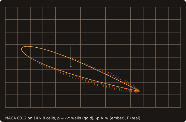
$ fig_ref_surface_loads_cut
cut pieces 115, wall segments 144, area A  0.081669
force  0.0000000  0.0816687   buoyancy (0, A)  0.0000000  0.0816687
moment about the leading edge: centroid values  0.0320783, with the gradient  0.0320760, A x_c  0.0320760
moment error: centroid values 2.4E-06;  with the gradient below 1e-15: T
Exact moments. The walls are flat, so the value at the centroid integrates a linear pressure exactly for the force: in p = p0 + g · x the force on a body inside the grid is −g V to round-off. The moment's integrand (x − c) p is then quadratic, and the centroid value misses the term ∫ (x − x_w)(x − x_w)ᵀ dA g = |A_w| K_w g of each wall (2.4·10⁻⁶ on a moment of 0.032 in the figure). With the pressure's gradient on each wall (gradient(d, n)) the sums add −(K_w g_w) × A_w and the moment is exact for a pressure linear on each wall: in 2-D K_w = d dᵀ / 12 from the segment d, in 3-D from cut_walls_gyration(walls, surface, x, y, z, gyration), which clips each term's polygon again with the cut's own clip (cut_wall_polygon_3d, the same polygon bit for bit) and sums its fans' exact second moments about the stored centroid. Without gradient the pressure is constant on each wall, a cell value, whose moment the centroid gives exactly too.
The checks (fossil_test_cut_loads_3d, _2d): bodies inside the grid (cube-01 on a grid through its faces and on one off them, an icosphere moved to a pose, two boxes, an irregular tetrahedron; a 64-gon, a disc with a hole, a NACA 0012 polygon plain and turned, two discs):
- buoyancy through the cut: F = −g V and, with the gradient, M = V (x_c − c) × (−g), within ε times the sum of the absolute terms (largest 0.10 / 0.05 of it in 3-D, 0.07 / 0.06 in 2-D); the centroid values alone miss the moment by 7·10⁻⁵ (3-D) and 2·10⁻⁶ (2-D) of that sum;
- a uniform pressure: the vector areas sum to 0;
- the walls of each piece sum to its
piece_wet_normal: bit for bit on every 2-D piece and on 1128 of 1602 3-D pieces; on the others the cut adds the fans in another association, and the sums agree within 1.7 ε times the piece's wall area; - FD and FV agree: the same linear p by
integrate_loadson samples of order 2 and by the cut walls gives the same force and moment, within ε times the two sums of absolute terms (largest 0.18); - a uniform shear gives τ times the area; per patch and per body sums add up, each box (disc) its own buoyancy.
call cut_cells_3d(sphere, x + 0.1_R8P, x, x - 0.1_R8P, cut, walls=walls)   ! the cut and its wall terms
p = 1._R8P - walls%centroid(3, :)                                 ! the pressure at the walls' centroids
call cut_loads_3d(walls, force, m0, pressure=p, about=[0._R8P, 0._R8P, 0._R8P], area=area)
call cut_walls_gyration(walls, sphere, x + 0.1_R8P, x, x - 0.1_R8P, gyration)   ! for the exact moment
g = spread([0._R8P, 0._R8P, -1._R8P], 2, walls%n)                 ! the pressure gradient on every wall
call cut_loads_3d(walls, force, m1, pressure=p, gradient=g, gyration=gyration, about=[0._R8P, 0._R8P, 0._R8P])
$ ref_surface_loads_cut
wall terms 8559, fluid pieces 12253; wetted area 3.1262326, V 0.5187371
force 0.0000000 0.0000000 0.5187371 error to (0, 0, V) 4.4E-18
moment, centroid values 0.1037446 -0.1556225 -0.0000009 error 2.8E-06
moment, with the gradient 0.1037474 -0.1556211 0.0000000 = V x_c x (0, 0, 1) to 1e-15: T
load samples (FD) = cut walls (FV) to 1e-15: T
per piece: force 0.0000337 0.0000532 0.5349629 error 1.6E-02The last line takes one pressure per fluid piece, at the piece's fluid centroid, as a cell-centred solver stores it: the force is then that of a piecewise-constant field, off by 3 % on 24³ cells. The value a wall needs is the one at the wall: reconstruct it (the cell value plus the gradient times x_w − x_cell) before the sum; FOSSIL does not.
call cut_cells_3d(surface, x, y, z, cut [, status], walls=walls)
call cut_walls_gyration(walls, surface, x, y, z, gyration [, status])
call cut_loads_3d(walls, force, moment [, status] [, pressure | pressure_per_piece] [, shear] [, gradient, gyration]
                  [, about] [, surface] [, per_patch_force] [, per_patch_moment] [, per_body_force] [, per_body_moment]
                  [, area] [, unassigned])
call curve%cut_cells(x, y, cut2 [, status], boundaries=.true.) ; call cut_walls_2d(cut2, walls2 [, status])
call cut_loads_2d(walls2, force, moment [, status] [, pressure | pressure_per_piece] [, shear] [, gradient] [, about]
                  [, curve] [, per_patch_force] [, per_patch_moment] [, per_body_force] [, per_body_moment] [, area])
p = cut_loads_linear_pressure(points, p0, gradient)- The walls inside the grid only. The terms cover the body where it lies in the grid's box: a body that leaves it loses those loads.
- Terms of no piece. In a cell without trusted pieces (3-D
pieces = -1, an open surface) a term has piece 0: withpressure_per_pieceit takes no pressure, andunassignedcounts it (one stderr line). Give such walls a pressure of their own throughpressure. - Refusals (
STATUS_INVALID_INPUT, zero outputs, per-patch / per-body arrays of size 0, a stderr line): no pressure and no shear, both pressures, a size that differs,gradientwithoutgyration(3-D) or without a pressure, per patch or per body without the surface (curve);cut_walls_2don a cut without boundaries;cut_walls_gyrationon another grid or surface. - CPU only, free routines of
fossil_cut_loads, re-exported byuse fossil. The device computes the wall terms (cut_cells_3d_device(..., walls=)); copy them back (update_host) before the sum.
What accuracy to expect
Both paths integrate over the faceted wall, so two questions decide what a solver gets: are the sums exact where the mathematics says they should be, and how fast does the faceted wall's force approach the smooth body's? The validation program fossil_val_surface_loads (a quadrature study, no flow solve: the pressure is given in closed form) answers both, through the load samples (integrate_loads, the FD path) and the cut walls (cut_loads_2d / _3d, the FV path).
Buoyancy on large meshes. In p = p0 + g · x the force is −g V and the moment V (x_c − c) × (−g) on any closed faceted body, V and x_c from mass_properties. The error, in units of ε times the sum of the absolute terms (as in the tests), on an icosphere of 81 920 facets with its vertices moved along the sphere (no symmetry) at a pose, a marching-cubes torus of 37 440 facets at a pose, a NACA 0012 of 4 000 segments and an ellipse of 8 192 (FV: 64³ cells, 2-D 512², with the gradient and, in 3-D, the walls' gyration):
| Body | Elements | FD q = 1, F | q = 2, F | q = 2, M | q = 3, F | q = 3, M | FV, F | FV, M |
|---|---|---|---|---|---|---|---|---|
| icosphere, stretched, posed | 81 920 | 0.04 | 0.04 | 0.03 | 0.04 | 0.02 | 0.04 | 0.02 |
| marching-cubes torus, posed | 37 440 | 0.03 | 0.03 | 0.04 | 0.03 | 0.07 | 0.03 | 0.07 |
| NACA 0012, 10° | 4 000 | 0.01 | 0.01 | 0.01 | 0.01 | 0.01 | 0.01 | 0.02 |
| ellipse 0.6 × 0.25, turned | 8 192 | 0.29 | 0.29 | 0.23 | 0.29 | 0.23 | 0.29 | 0.23 |
The sums stay exact to round-off at any size: the compensated sums keep the error of the terms, not of their number. The order-1 moment and the FV moment without the gradient are not exact (a quadratic integrand): off by 8·10⁻⁸ and 5·10⁻⁸ of the sum on the icosphere. The bunny, the dragon and dragon-fine are not watertight: they have no volume to compare with and are skipped.
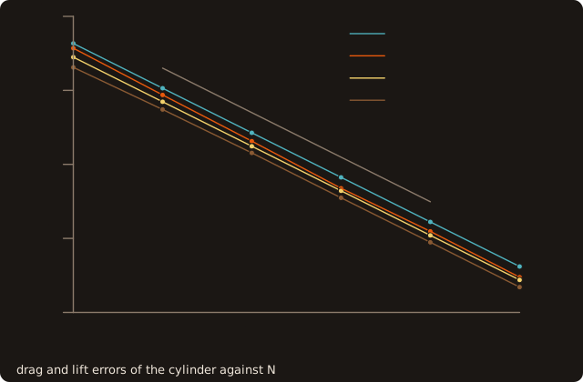
Potential flow. A cylinder of radius R = 0.5 in a uniform flow U = 1 with circulation Γ = −0.8 (2π U R) has zero drag (d'Alembert) and lift −ρ U Γ (Kutta–Joukowski); a sphere in a uniform flow has zero force. The pressure is p = p∞ + ρ (U² − |u|²) / 2 with u the exact velocity on the true wall at the point nearest the sample (the radial projection), the convention of the closure's validation: the solver imposes the smooth body's data on the faceted wall, so the error is that of the facets and of the rule alone. The walls are polygons and icospheres with their vertices on the circle and the sphere, moved along them towards a point so that no symmetry cancels the drag. The figure: the cylinder through both paths, the FD path with samples of order 2, the FV path on N/2 cells per axis:
call load_samples_2d(wall, samples=ls, order=2_I4P)                 ! FD: the load samples of order 2
p = [(pressure(ls%points(:, i)), i = 1, ls%n)]                      ! p of the true wall at each sample
call integrate_loads(ls, f, m, pressure=p)
e(k, 1) = abs(f(1)) / (RHO * U**2 * R) ; e(k, 2) = abs(f(2) - LIFT) / abs(LIFT)
h = 1.6_R8P / (n / 2)                                               ! FV: n / 2 cells per axis
x = [(ZC(1) - 0.8_R8P + 0.31_R8P * h + i * h, i = 0, n / 2)]
y = [(ZC(2) - 0.8_R8P + 0.17_R8P * h + i * h, i = 0, n / 2)]
call wall%cut_cells(x, y, cut, boundaries=.true.)
call cut_walls_2d(cut, walls)                                       ! the wall segments of the cut pieces
p = [(pressure(walls%centroid(:, i)), i = 1, walls%n)]              ! p of the true wall at each midpoint
call cut_loads_2d(walls, f, m, pressure=p)
e(k, 3) = abs(f(1)) / (RHO * U**2 * R) ; e(k, 4) = abs(f(2) - LIFT) / abs(LIFT)
$ fig_ref_surface_loads_accuracy
cylinder R = 0.5, U = 1, Gamma = -0.8 (2 pi U R): errors |F_x| / (rho U^2 R) and |F_y - L| / |L|
N FD drag FD lift FV drag FV lift (FD: order-2 samples; FV: N / 2 cells per axis)
32 4.30E-03 2.81E-03 3.72E-03 2.04E-03
64 1.07E-03 7.02E-04 8.66E-04 5.51E-04
128 2.67E-04 1.76E-04 2.06E-04 1.43E-04
256 6.67E-05 4.39E-05 4.76E-05 3.53E-05
512 1.67E-05 1.10E-05 1.24E-05 8.85E-06
1024 4.17E-06 2.74E-06 2.98E-06 2.19E-06
order 2.00 2.00 2.06 2.01From the validation (errors |F_x| / (ρ U² R), |F_y − L| / |L| in 2-D, |F| / (ρ U² π R² / 2) in 3-D; h_s the longest segment or edge; the observed order of the two finest levels in the last row):
| N | h_s | drag, q = 1 | q = 2 | q = 3 | lift, q = 1 | q = 2 | q = 3 |
|---|---|---|---|---|---|---|---|
| 32 | 1.4e-1 | 1.6e-3 | 4.3e-3 | 4.3e-3 | 1.8e-3 | 2.8e-3 | 2.8e-3 |
| 256 | 1.8e-2 | 2.6e-5 | 6.7e-5 | 6.7e-5 | 2.9e-5 | 4.4e-5 | 4.4e-5 |
| 4 096 | 1.1e-3 | 1.0e-7 | 2.6e-7 | 2.6e-7 | 1.1e-7 | 1.7e-7 | 1.7e-7 |
| order | 2.00 | 2.00 | 2.00 | 2.00 | 2.00 | 2.00 |
| Icosphere level | Facets | h_s | q = 1 | q = 2 | q = 3 |
|---|---|---|---|---|---|
| 1 | 80 | 4.2e-1 | 2.8e-2 | 4.0e-2 | 3.9e-2 |
| 4 | 5 120 | 5.8e-2 | 4.7e-4 | 6.9e-4 | 6.9e-4 |
| 6 | 81 920 | 1.5e-2 | 2.9e-5 | 4.3e-5 | 4.3e-5 |
| order | 2.01 | 2.01 | 2.01 |
| FV | Cells | h | Drag (2-D) / force (3-D) | Lift | FD (q = 3) − FV |
|---|---|---|---|---|---|
| cylinder, N = 2 n | 64² | 2.5e-2 | 2.1e-4 | 1.4e-4 | 1.7e-4 |
| 1 024² | 1.6e-3 | 7.5e-7 | 5.5e-7 | 7.0e-7 | |
| order | 1.99 | 2.00 | 1.99 | ||
| sphere, level 1 + log₂(n/4) | 16³ | 1.0e-1 | 2.4e-3 | 3.7e-4 | |
| 64³ | 2.5e-2 | 1.5e-4 | 2.8e-5 | ||
| order | 1.98 | 2.08 |
- Second order in the facet size, set by the facets. Every error falls as h_s², through both paths, in 2-D and 3-D: the faceted wall's normals and areas carry an O(h_s²) error of the force.
- The rule is not the limit. Orders 2 and 3 agree to three digits: their own quadrature error is far below the facets'. Order 1 comes out 1.4–2.6 times smaller, because its O(h_s²) rule error happens to cancel part of the facets' here; a cancellation, not a property to count on. Refine the facets, not the rule (Limitations).
- FD and FV agree to the discretisation error. On the same faceted wall the FD path with order 3 is the facets' exact integral to O(h_s⁶); the FV path takes the value at the centroid of each wall fragment, a midpoint rule, so their difference is that rule's error, of order 2 (1.99 in 2-D, 2.08 in 3-D): of the size of either path's error to the smooth body in 2-D, a fifth of it in 3-D.
- Which flow at the sample. The flow continued analytically to the sample point, inside the true body, gives the same order with another constant (cylinder at N = 4 096: drag 6.6·10⁻⁷, lift 7.8·10⁻⁸; sphere at level 6: 1.2·10⁻⁴); a solver has no flow there, so the validation uses the true wall's.
Pass criteria of fossil_val_surface_loads (it prints Are all tests passed? T iff all hold, about 4 s at -O2, 0.4 GB): the buoyancy force within 1 (units of ε times the sum of the absolute terms) on every body, path and rule order, the moment within 1 where it is exact (FD from order 2, FV with the gradient and the gyration); the d'Alembert and Kutta–Joukowski errors and the FD − FV difference decreasing at an observed order of at least 1.8 over the two finest levels, for every rule order and on the cut walls.