
Cut cells: solver support
FOSSIL's cut cells give a block's fluid fractions, apertures, centroids, wall measures and fluid pieces. A conservative cut-cell solver needs more geometry before its first step: the neighbourhoods its small-cell cure works on, merge targets for small, fresh and dead cells, moments above the first, coarse levels, and the fluid fractions of the cell edges. Issue #70 (roadmap #68, WP1) adds them as pure geometry and graph work; the solver keeps the arithmetic on its states and fluxes.
Design and reference (issue #70)
Each section says what the literature prescribes, with the source, what FOSSIL chooses where the literature leaves room, the interface, and what the tests measured. Statements from general knowledge rather than a cited source are marked (gk). A worked example is in the cookbook: Neighbourhoods for a small-cell cure.
At a glance
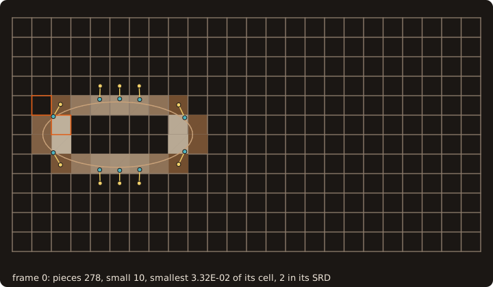
Each frame recomputes the cut cells of a moving ellipse, their links, the state-redistribution neighbourhoods and the merge targets: 8 to 13 small pieces per frame (area below half the cell), the smallest down to 2.61e-05 of its cell (anim_cut_solver.f90).
Principles
- The piece is the unit. Every neighbourhood, link and target is indexed by the pieces
1..cut%np, not by cells. A cell with one piece is that piece; a regular cell is one piece with κ = 1. AMReX's embedded boundaries are single-valued per cell (gk); a thin plate across a cell gives FOSSIL two pieces with two states, and the graph keeps them apart. - Trusted cells only. A cell with
pieces = -1has no pieces, so it takes no part in the graph; its neighbours see it as a wall. Every output reports such gaps through a status, never through a silent fallback. - Zero-volume pieces carry no state. A wall on the high plane of a cell leaves a fluid face bounding no fluid volume (limitations). These pieces get links (their face is open) but are never members, centres or targets of a neighbourhood; a solver treats their faces as walls.
- Deterministic. Every choice follows a fixed order on (cell index in x-fastest order, piece index): the same input gives the same output, with or without OpenMP.
- CPU only. The cut cells are computed on the CPU, and this is preprocessing per block, not a batched point query: no device path.
- New free modules, the cut-cell types unchanged in shape:
fossil_cut_graph(links, neighbourhoods, targets),fossil_cut_moments(moments, quadrature),fossil_cut_coarsen(coarse levels). The links and moments need the transient wall polygons ofcut_cells_3d, so it takes optional arguments that compute them only when asked.
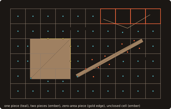
The 60 cells hold 60 pieces: 37 regular cells, 5 cells with two pieces, 3 pieces of zero area where the square's sides lie on the high edges of their cells (their only fluid is the open edge), and 4 cells the open curve leaves unclosed, with no pieces at all; in 2-D an unclosed cell has closed false, in 3-D pieces = -1 (fig_ref_cut_solver_pieces.f90).
The piece graph
A link (p, q, f, A) says that piece p of cell c and piece q of the cell across face f of c share a fluid region of that face, of area A. It is stored from p's side in CSR form (cut_links_t): start(np + 1), piece(:), face(:) (1 to 6: −x, +x, −y, +y, −z, +z; 1 to 4 in 2-D) and area(:), sorted by face, then by the piece across. Both directions are stored, with the same area.
x = [(-0.5_R8P + 0.25_R8P * i, i = 0, 8)]
call cube%load_from_file(file_name='cube-01.stl', guess_format=.true.)           ! [0, 1]^3 on the cell faces
call cut_cells_3d(cube, x, x, x, cut3, links=links3, edges=.true.)             ! 3-D: links with the cut cells
print '(A,I0,A,I0,A,I0,A,I0)', '3-D: pieces ', cut3%np, ' (', count(cut3%piece_volume == 0._R8P), &
                               ' of zero volume), links ', size(links3%piece), ', unmatched regions ', links3%unmatched
p = 1
do k = links3%start(p), links3%start(p + 1) - 1 ! piece p meets piece(k) over its face face(k), area area(k)
   print '(A,I0,A,I4,A,I0,A,F7.4)', '  piece ', p, ' -> ', links3%piece(k), ' over face ', links3%face(k), &
                                    ', area ', links3%area(k)
enddo
print '(A,I0,A,I0)', '  z edges with fluid ', count(cut3%edge_z > 0._R8P), ' of ', size(cut3%edge_z)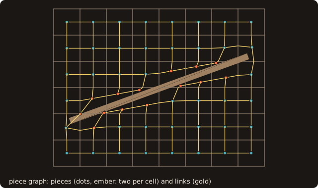
The plate splits 7 of the 48 cells: 55 pieces, 176 links counted in both directions, none across the plate (fig_ref_cut_solver_links.f90).
- 2-D. The fluid intervals of a cell edge are bounded by the crossings of the walk and the cell corners, the same points in the two cells that share the edge, so the intervals of two pieces across an edge are equal or disjoint: one link per pair of equal intervals, of their length. The cut cells now also give each piece's apertures (
piece_aperture(4, np)) and its fluid intervals (piece_iv_start,piece_iv_edge,piece_iv_lo,piece_iv_hi). - 3-D. A connected fluid region of a face lies next to one piece on each side. The regions are the pieces of the plane section's 2-D cut cell (their areas are the same numbers as the face fractions), matched to the 3-D pieces on both sides through the fluid edge intervals they share, the edges of the face being cell edges. A one-piece side takes every region; two one-piece cells get one link of the face's fluid area. A region with no fluid interval (a fluid island inside a solid trace on the face) goes to the only piece of its side whose face area it leaves unexplained, else it is counted in
links%unmatchedand gets no link. - Untrusted cells (
pieces = -1) have no pieces and no links: their neighbours see a wall there.
Measured (fossil_test_cut_links, fossil_test_cut_links_3d):
| Case | Result |
|---|---|
| 2-D: circle on a generic and an aligned grid, thin plate | link sums = piece aperture × edge length to 1·10⁻¹⁶, exact symmetry, per-piece apertures add up to the cell's exactly; plate pieces never link across the plate |
| 3-D: tilted wedge, cone, L-prism (generic, aligned), thin plate, square tube (hole as a face island), 8 lattice tetrahedra; 113 298 links, 193 multi-piece cells | link sums = piece face fraction × face area to 1.2·10⁻¹⁴, exact symmetry, 0 unmatched regions; plate pieces never link across the plate |
| links on the device vs the host: 3-D bench bodies, sphere and cone at 64³; 2-D ellipse, NACA 0012, 50 circles at 256² and 1024²; copied back and resident | every field bit for bit (cut links 3-D / 2-D device vs serial mismatches, fossil_test_cut_links_3d_twin, fossil_test_cut_links_2d_twin) |
On the device
The links are built per face (per edge in 2-D) and per piece, with no global sort: each face fills slots of (low piece, high piece, area) after a count and a prefix sum, and a per-piece pass emits the CSR in (face, piece across) order, adding equal keys in the order the regions of their face come. The result is the same cut_links_t bit for bit as the sort-based assembly it replaced, and the cost grows with the cells (N³), not with N^3.7-4.0.
On the device:
cut_cells_3d_device(surface, x, y, z, cut, links=, resident=)computes the cut, keeps the fluid edge intervals of the pieces and the plane sections resident, and runs the link stage there;cut_links_2d_device(cut, links, resident)does the 2-D links from a resident or hostcut_cells_2d_t.
Both return the links copied back or, with resident=.true., mapped on the device (links%update_host, links%exit_device, the cut cells' contract). Measured on an RTX 4070, best of 5 after a warm-up:
| case | CPU, cut + links [s] | device, resident [s] | device, copied back [s] |
|---|---|---|---|
| sphere, 128³ | 1.44 | 0.153 | 0.347 |
| cone, 128³ | 1.35 | 0.205 | 0.369 |
| ellipse, 1024² | 0.125 | 0.011 | 0.035 |
| NACA 0012, 1024² | 0.149 | 0.012 | 0.044 |
The link stage itself adds 1-6 % to the device cut cells. SRD, FRD and the merge targets read the links on the host.
Neighbourhoods for state redistribution
State redistribution (Berger & Giuliani 2021, §4; llm-wiki high-order-capturing-schemes/wiki/methods/state-redistribution.md) merges each small cell with neighbours "preferably in the direction of the wall normal" until the merged volume reaches ½ hᵈ, falling back to a centred 3ᵈ, then 5ᵈ, tile. The rule for choosing neighbours inside the tile is left open; FOSSIL's is:
- A piece p is small if |I_p| < τ hᵈ (τ = ½ by default, an argument; the threshold is a 1-D stability result, unproved in 2-D and 3-D, by the authors' own account). A piece that is not small has N_p = {p}.
- Candidates are the pieces of the 3ᵈ tile around p's cell reachable from p through links between pieces of the tile, zero-volume pieces excluded.
- Order: by the alignment of the cell offset o ∈ {−1, 0, 1}ᵈ with the unit wall normal n̂ of p (into the fluid), s = n̂ · o / |o|, largest first; ties by smaller |o|₁, then lexicographic o, then piece index.
- Growth: candidates join in that order until Σ |I_j| ≥ τ hᵈ. If the 3ᵈ tile is exhausted, the 5ᵈ tile is used with the same rule; if that is exhausted too, the neighbourhood is kept with status incomplete.
- Outputs: the neighbourhoods in CSR form (p first), the overlap counts N^ov_j (the neighbourhoods containing j, its own included), the weighted volumes V̂_p = Σ_{j∈N_p} |I_j| / N^ov_j and centroids x̂_p, and the weighted factors of Giuliani et al. 2022 (§3.1): η^nb_p = (τ hᵈ − |I_p|) / Σ_{j∈N_p∖p} |I_j| for small p, else 0, and η^self_p = 1 − (1/N^ov_p) Σ_{k≠p, p∈N_k} η^nb_k.
- Each neighbourhood depends on its own piece only, so the result does not depend on the order in which pieces are visited.
h = [(0.1_R8P * i, i = 0, 10)] ! 10 x 10 cells of 0.1; the solid is x < 0.58: fluid fraction 0.2 in the cut column
call half%adopt_loops(u=[-1._R8P, 0.58_R8P, 0.58_R8P, -1._R8P], v=[-1._R8P, -1._R8P, 2._R8P, 2._R8P], loop_sizes=[4_I4P])
call half%cut_cells(x=h, y=h, cut=cut, moments_order=2_I4P)
call cut_links_2d(cut, links)                                                  ! 2-D: from the cut cells
call srd_neighbourhoods(links, cut%piece_cell, cut%piece_area, cut%piece_centroid, cut%piece_wet_normal, h, h, srd)
print '(A,I0,A,I0,A,I0)', '2-D: pieces ', cut%np, ', small ', count(srd%status == SRD_COMPLETE), ', regular ', &
                          count(srd%status == SRD_REGULAR)
p = minloc(cut%piece_area, 1, mask=cut%piece_area > 0._R8P .and. cut%piece_cell(2, :) == 5)
print '(A,2I3,A,F5.2,A,10I4)', '  piece in cell', cut%piece_cell(:, p), ', fraction ', cut%piece_area(p) / 0.01_R8P, &
                               ', SRD members', srd%member(srd%start(p):srd%start(p + 1) - 1)
print '(A,2I3,A,F6.3,A,F6.3)', '  member cells', cut%piece_cell(:, srd%member(srd%start(p) + 1)), &
                               ', eta_nb ', srd%eta_nb(p), ', eta_self ', srd%eta_self(p)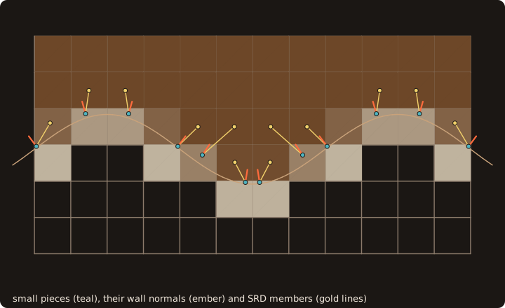
On the wavy wall 12 of the 46 pieces are small; every neighbourhood is complete with one neighbour (2 members), the neighbour chosen along the wall normal. Σ V̂ equals the fluid area to 0.00e+00 and η^nb ranges from 0.022 to 0.651 (fig_ref_cut_solver_srd.f90).
Measured (fossil_test_cut_srd; 2-D circle, thin plate and half-plane, 3-D tilted wedge, cone and thin plate, τ = ½, 327 small pieces): every piece with volume is in exactly N^ov_j neighbourhoods and the column sums are 1 exactly; Σ V̂ is the total fluid volume to 10⁻¹⁴; x̂ is the weighted centroid of the members to round-off; no neighbourhood is incomplete; 0 ≤ η^nb ≤ 1 and 0 < η^self ≤ 1; on the half-plane x < 0.58 (cells of 0.1, fraction 0.2) every small cell merges with the cell across its +x face only, the wall normal; no neighbourhood crosses a plate.
Neighbourhoods for flux redistribution
Flux redistribution (llm-wiki methods/flux-redistribution.md; Natarajan et al. 2022 §2; Barrio Sanchez et al. 2024 App. A) averages over the fluid cells of the 3ᵈ block around a cut cell "that can be reached from it", made precise by Barrio Sanchez et al. as a monotone index path through valid cells.
- Path: from p, a sequence of links each of which moves one index by one step towards the target cell's offset, never away, through pieces that are trusted and have volume.
- Weights: κ_j / Σ κ over the reached set, p included (κ = |I| / hᵈ).
- A piece filling its cell has itself only, weight 1; a zero-volume piece has no set.
frd_neighbourhoods(links, piece_cell, piece_volume, x, y, frd, z=)givesfrd_t(start,memberwith the piece first,weight).
call frd_neighbourhoods(links, cut%piece_cell, cut%piece_area, h, h, frd)
print '(A,I0,A,F6.3)', '  FRD set size ', frd%start(p + 1) - frd%start(p), ', own weight ', frd%weight(frd%start(p))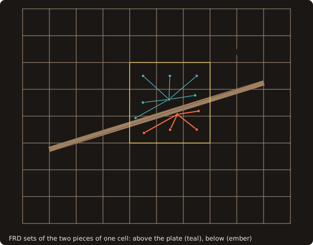
The split cell (6, 5) holds a piece above the plate, fraction 0.741, and one below, fraction 0.068. Their sets have 7 and 5 members, own weights 0.142 and 0.021: both lie in the same 3 × 3 block, but no monotone path of links crosses the plate (fig_ref_cut_solver_frd.f90).
- Measured (
fossil_test_cut_frd; 2-D circle and thin plate, 3-D tilted wedge and thin plate, 654 cut pieces): every set equals a brute-force fixpoint that pulls pieces in from the cell grid (a formulation independent of the library's breadth-first search); the weights sum to 1 to 8.9·10⁻¹⁶; no set crosses a plate where the block lies within the plate (near its ends a monotone path goes around).
Merge targets
Two families, both reported per piece:
- One target (cell merging; Falcovitz et al. 1997 in llm-wiki
methods/cut-cell-finite-volume.md: covered, newly exposed and small cells merge "with an adjacent wet cell"). The target is the linked piece, not small, that maximises n̂ · o / |o|, ties by the larger link area, then the lower index. When every linked piece is small, the chain is followed to the first piece that is not; a cycle is reported. - Normal-directed targets (conservative mixing; Bezgin et al. 2023 §3.6 in llm-wiki
weno-teno/wiki/methods/level-set-method.md: "up to seven target cells in 3D chosen from the interface normal"). The targets are the pieces at the offsets o with o_a ∈ {0, sign n_a}, o ≠ 0 (3 in 2-D, 7 in 3-D), reached by a monotone path. The weights of the cited scheme are not in the wiki; FOSSIL reports β_o ∝ (Π_{a: o_a ≠ 0} |n_a|)^{2/|supp o|} (gk, after Hu et al. 2006), normalised over the targets found, and leaves the volume-fraction factor to the solver. - Fresh and dead pieces of a moving body come from
swept_cells_2d/3d(cleared,covered): the caller passes the pieces to serve as a mask and the pieces that may not serve as targets (for a dead piece, the pieces of the covered cells), and the same rules apply on the cut cells at the right pose. A target that switches on or off between steps changes the discrete operator abruptly: Schneiders et al. (2013, §4-§6) measure drag jumps from it in a conservative merged scheme, while Seo & Mittal (2011) and Xie et al. (2022) find that conservation alone removes most oscillations (an open disagreement in the llm-wiki). - A piece is suitable as a target if it has volume, is not small and is not excluded. An unsuitable single target (a small one, or a dying neighbour of a dying piece) starts a chain followed to the first suitable piece (
final_target, statusMERGE_CHAIN); a chain that loops or ends is reported (MERGE_CYCLE), a piece with no linked piece with volume too (MERGE_ALONE). merge_targets(links, piece_cell, piece_volume, wet_normal, x, y, mt, z=, tau=, mask=, exclude=)givesmerge_t(status,target,final_target,mix_start,mix_piece,mix_weight).
call merge_targets(links, cut%piece_cell, cut%piece_area, cut%piece_wet_normal, h, h, mt)
if (mt%status(p) == MERGE_OK) print '(A,2I3,A,I0,A,F5.2)', '  merge target in cell', cut%piece_cell(:, mt%target(p)), &
   ', normal-directed targets ', mt%mix_start(p + 1) - mt%mix_start(p), ', weight ', mt%mix_weight(mt%mix_start(p))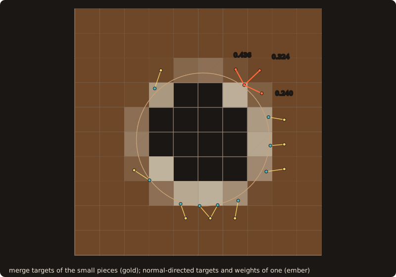
Around the disc 10 of the 88 pieces are small and all 10 merge directly (MERGE_OK, no chain). The piece of cell (7, 7), fraction 0.052, has a wall normal near the diagonal: its three normal-directed targets carry 0.240, 0.436 and 0.324 (fig_ref_cut_solver_merge.f90).
- Measured (
fossil_test_cut_merge; 2-D half-plane, circle and a translating circle, 3-D tilted wedge, 250 served pieces): on the half-plane x < 0.58 every small cell targets the cell across its +x face, also as its only normal-directed target, weight 1; every target is linked and suitable or ends a chain at a suitable piece; normal-directed targets lie at the offsets with o_a ∈ {0, sign n_a}, at most 2ᵈ − 1, in distinct cells, weights summing to 1 to 2.2·10⁻¹⁶; the 15 fresh pieces of the moving circle (at the end pose) and its 18 dead ones (at the start pose, the covered cells excluded) all get targets, no cycle and no lone piece.
Moments and quadrature
- Moments of a piece: ∫ ((x − x_c)/h_x)^a ((y − y_c)/h_y)^b ((z − z_c)/h_z)^c dV for a + b + c ≤ p (p ≤ 4), about the cell centre x_c, scaled by the cell size so they stay O(|I|) far from the origin; the same for the face fluid regions and the wall polygons. Volume moments by the divergence theorem along x, ∫_V x^α dV = (1/(α_x + 1)) ∮ x^{α + e_x} n_x dA: the wall polygons (fan triangles, a rule exact to degree p + 1) and the +x face only (local coordinates put the −x face at 0); face moments by Green's theorem over the same boundary arcs as the face fractions; 2-D by Green. First moments must equal the existing centroids.
- Interface:
cut_cells_3d(..., moments_order=p)givespiece_moments(:, np),piece_wall_moments(:, np),piece_face_moments(:, 6, np)and the face totalsface_x/y/z_moments, in the order ofmono_exponents(fossil_cut_moments: by degree, then decreasing exponent of X, then of Y); 2-Dcurve%cut_cells(..., moments_order=p)givespiece_momentsandpiece_wall_moments. The faces of a one-piece cell come from the plane sections (the same numbers as the face fractions), those of a multi-piece cell from the same boundary arcs as its face areas; a fluid cell is analytic. Kernels: 3-point Gauss on segments and the symmetric 7-point triangle rule in closed form, both exact to degree 5. - Measured (
fossil_test_cut_moments, order 4): summed over the pieces and re-centred to global monomials, the moments equal the block's minus the body's (integrated independently over tetrahedra from the origin) to 9.9·10⁻¹⁴ relative on the tilted wedge, the aligned L-prism and the thin plate, and to 3.6·10⁻¹⁵ in 2-D (a 64-gon); the zeroth and first moments equal the piece volumes and centroids, the wall ones the wetted areas and centroids (2.0·10⁻¹⁵ of the cell); the face moments of the pieces add up to the plane sections' (5.7·10⁻¹⁵ of the face). The moments do not depend on the order of the loops (fossil_test_cut_moments_order, issue #95: up to v3.0.0 a cell joining three or more wall chains lost the moments of a chain charged to a root that a later union absorbed): four corner squares in all 24 loop orders agree to 1.2·10⁻¹⁷ relative and with the closed form to 4.4·10⁻¹⁶; in 3-D the zeroth moments equal the piece volumes to 2.4·10⁻¹⁵ of the cell. - Quadrature (
cut_cells_3d(..., quadrature=.true.), 2-Dcurve%cut_cells(..., quadrature=.true.)): per piecequad_start,quad_point,quad_weight, andwall_quad_start,wall_quad_point,wall_quad_weight; 3-Dquad_status(0: the weights add up to the piece volume).- Wall rules: the symmetric 7-point rule on the wall fan triangles (3-D), 3-point Gauss on the wall segments (2-D); positive weights, exact to degree 5.
- Volume rules: signed cones from the cell centre over the oriented fluid boundary of the piece (gk: the divergence-theorem cone construction): the wall fans reversed and, on every face, the triangles from the face centre to the face region's oriented boundary, from the plane section for a one-piece cell (exact, as the face fractions) and from the face arcs of the pieces otherwise; 36 points per cone (Duffy map, Gauss 4 × 3 × 3), exact to degree 4; a fluid cell takes the 3ᵈ Gauss rule. Weights are negative where a piece is not star-shaped about the cell centre: they are counted, not hidden. 2-D: signed triangles from the cell centre over the exported oriented boundary (
boundaries=.true.:piece_seg_start,piece_seg,piece_seg_wall). - Measured (
fossil_test_cut_quadrature; L-prism generic and aligned, thin plate, 4 lattice tetrahedra, a 64-gon; 5028 pieces): the rules integrate every monomial of degree ≤ 4 to the piece's moments to 4.8·10⁻¹⁵ of the cell, the wall rules to 1.4·10⁻¹⁵; 360 pieces have negative volume weights; 1 piece hasquad_status1, a two-piece cell of a lattice tetrahedron whose face arcs (the clipped traces, as its face areas) do not close.
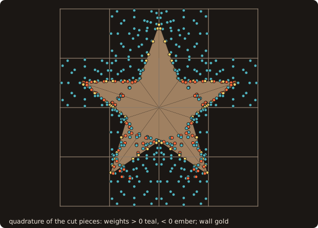
On the star, 14 of the 20 pieces are cut; their rules have 544 volume points, 98 of them with a negative weight, and 72 wall points. The weights of every piece add up to its area within 3.82e-17 (fig_ref_cut_solver_quadrature.f90). A signed triangle from the cell centre covers what lies between the centre and the boundary, solid included: its points can lie outside the piece, and the triangles over the solid side carry the negative weights that cancel them.
Coarsening
Coarse–fine cut cells are where re-redistribution fails at κ < 10⁻⁴ (llm-wiki methods/high-order-amr.md). The coarse geometry at ratio r (nested edges, the cell counts multiples of r) is built from the fine one, never recomputed: cut_coarsen_3d(fine, links, x, y, z, ratio, coarse, coarse_links, fine_to_coarse, status) (2-D cut_coarsen_2d, without z).
- Coarse pieces are the connected components of the fine pieces of a coarse cell, joined by the fine links inside it;
fine_to_coarsemaps every fine piece to its coarse one. - Volumes, centroids, wetted measures, the fluid areas of the coarse faces, the moments (re-centred and rescaled to the coarse cell) and the links are sums of the fine ones; node flags and edge fractions come from the fine ones. A coarse cell with an untrusted fine cell is untrusted. Face piece counts are not derived (−1); quadrature rules are not coarsened (concatenating the fine rules is exact).
call cut_coarsen_2d(cut, links, h, h, 2_I4P, coarse, coarse_links, fine_to_coarse, status)
print '(A,I0,A,I0,A,I0,A,F5.2)', 'coarse (ratio 2): status ', status, ', pieces ', coarse%np, ', links ', &
                                 size(coarse_links%piece), ', fraction of the cut column ', coarse%alpha(3, 3)
print '(A,I0,A,I0)', '  the fine piece lands in coarse piece ', fine_to_coarse(p), ', in coarse cell ', &
                     coarse%piece_cell(1, fine_to_coarse(p))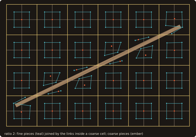
At ratio 2 the 106 fine pieces (10 cells with two) become 28 coarse ones (4 cells with two), and the 356 fine links 80 coarse ones; the coarse fluid area equals the fine one to 6.66e-16 (fig_ref_cut_solver_coarsen.f90).
- Measured (
fossil_test_cut_coarsen; tilted wedge, L-prism, thin plate, a 64-gon and a thin plate in 2-D; 2612 coarse cells at ratio 2): against the cut cells computed directly on the coarse grid, the same pieces in every cell, piece volumes to 2.5·10⁻¹⁴ of the cell, fractions and wetted areas to 2.5·10⁻¹⁴, node flags exactly, edge fractions to 1.1·10⁻¹⁶, moments to 1.2·10⁻¹⁵, link areas per coarse face to 7.8·10⁻¹⁵.
Edge fractions
cut_cells_3d(..., edges=.true.) gives the fluid fraction of every cell edge, edge_x(nx, ny + 1, nz + 1), edge_y(nx + 1, ny, nz + 1) and edge_z(nx + 1, ny + 1, nz) (one query per grid line, off by default: the swept geometry calls the cut cells many times and needs no edges). Every call gives the inside flag of every grid node, node_in(nx + 1, ny + 1, nz + 1) (the z lines); the 2-D cut cells give node_in(nx + 1, ny + 1) (their edges are the apertures). Embedded-boundary constrained transport needs the edge fractions (llm-wiki div-free-amr/wiki/methods/embedded-boundary-constrained-transport.md).
- Exact topology. Every grid line is queried once (
line_crossings). A crossing belongs to the segment between two nodes when it lies after the perturbed lower node and before the perturbed upper one (line_crossing_before, one exactorient3d, ties by the global perturbation of issue #69). The first node's flag is the parity of the crossings before it; the next ones flip at each crossing. Lengths use the rounded crossing positions. - The same node flags are the corner states of the 3-D pieces.
- Measured (
fossil_test_cut_edges): against the apertures of the plane sections' 2-D cut cells (a separate code path:slice_surfaceand the 2-D walk), on the tilted wedge, the L-prism (generic and aligned), cube-01 through its faces and 6 lattice tetrahedra: 209 132 edges agree to 4.3·10⁻¹⁵. Of 60 231 node flags, 7 differ, all at nodes exactly on the surface of a lattice tetrahedron, where the sections decide on rounded crossing points (limitations); the 3-D flags are exact predicates on the input triangles.
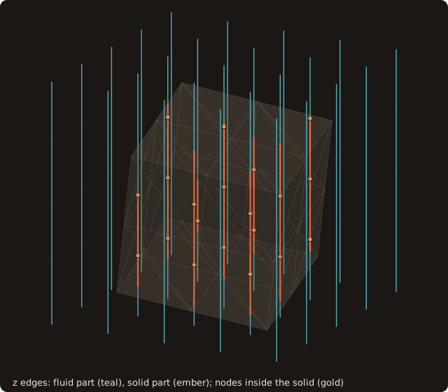
Of the 100 z edges, 71 are all fluid, 11 all solid and 18 cut; 20 of the 125 nodes are inside. Each cut edge has one crossing here, so its split point, placed at its fraction from its fluid node, lies on the cube to 2.63e-16 (fig_ref_cut_solver_edges.f90).
Example
The regions shown above, as one program: the cube-01 body on a 3-D block of 8³ cells of 0.25, then the half-plane x < 0.58 on 10 × 10 cells of 0.1 (the solid on the left, the fluid fraction of the cut column 0.2). The cookbook recipe Neighbourhoods for a small-cell cure does the same on a disc.
program ref_cut_solver
use fossil, only : surface_stl_object, curve_object, cut_cells_2d_t, cut_cells_3d_t, cut_cells_3d, cut_links_t, &
                   cut_links_2d, srd_t, srd_neighbourhoods, SRD_REGULAR, SRD_COMPLETE, frd_t, frd_neighbourhoods, &
                   merge_t, merge_targets, MERGE_OK, cut_coarsen_2d, mono_count
use penf,   only : I4P, R8P
implicit none
type(surface_stl_object)  :: cube
type(curve_object)        :: half
type(cut_cells_3d_t)      :: cut3
type(cut_cells_2d_t)      :: cut, coarse
type(cut_links_t)         :: links3, links, coarse_links
type(srd_t)               :: srd
type(frd_t)               :: frd
type(merge_t)             :: mt
real(R8P)                 :: x(9), h(11)
integer(I4P), allocatable :: fine_to_coarse(:)
integer(I4P)              :: i, k, p, status

x = [(-0.5_R8P + 0.25_R8P * i, i = 0, 8)]
call cube%load_from_file(file_name='cube-01.stl', guess_format=.true.)           ! [0, 1]^3 on the cell faces
call cut_cells_3d(cube, x, x, x, cut3, links=links3, edges=.true.)             ! 3-D: links with the cut cells
print '(A,I0,A,I0,A,I0,A,I0)', '3-D: pieces ', cut3%np, ' (', count(cut3%piece_volume == 0._R8P), &
                               ' of zero volume), links ', size(links3%piece), ', unmatched regions ', links3%unmatched
p = 1
do k = links3%start(p), links3%start(p + 1) - 1 ! piece p meets piece(k) over its face face(k), area area(k)
   print '(A,I0,A,I4,A,I0,A,F7.4)', '  piece ', p, ' -> ', links3%piece(k), ' over face ', links3%face(k), &
                                    ', area ', links3%area(k)
enddo
print '(A,I0,A,I0)', '  z edges with fluid ', count(cut3%edge_z > 0._R8P), ' of ', size(cut3%edge_z)

h = [(0.1_R8P * i, i = 0, 10)] ! 10 x 10 cells of 0.1; the solid is x < 0.58: fluid fraction 0.2 in the cut column
call half%adopt_loops(u=[-1._R8P, 0.58_R8P, 0.58_R8P, -1._R8P], v=[-1._R8P, -1._R8P, 2._R8P, 2._R8P], loop_sizes=[4_I4P])
call half%cut_cells(x=h, y=h, cut=cut, moments_order=2_I4P)
call cut_links_2d(cut, links)                                                  ! 2-D: from the cut cells
call srd_neighbourhoods(links, cut%piece_cell, cut%piece_area, cut%piece_centroid, cut%piece_wet_normal, h, h, srd)
print '(A,I0,A,I0,A,I0)', '2-D: pieces ', cut%np, ', small ', count(srd%status == SRD_COMPLETE), ', regular ', &
                          count(srd%status == SRD_REGULAR)
p = minloc(cut%piece_area, 1, mask=cut%piece_area > 0._R8P .and. cut%piece_cell(2, :) == 5)
print '(A,2I3,A,F5.2,A,10I4)', '  piece in cell', cut%piece_cell(:, p), ', fraction ', cut%piece_area(p) / 0.01_R8P, &
                               ', SRD members', srd%member(srd%start(p):srd%start(p + 1) - 1)
print '(A,2I3,A,F6.3,A,F6.3)', '  member cells', cut%piece_cell(:, srd%member(srd%start(p) + 1)), &
                               ', eta_nb ', srd%eta_nb(p), ', eta_self ', srd%eta_self(p)

call frd_neighbourhoods(links, cut%piece_cell, cut%piece_area, h, h, frd)
print '(A,I0,A,F6.3)', '  FRD set size ', frd%start(p + 1) - frd%start(p), ', own weight ', frd%weight(frd%start(p))

call merge_targets(links, cut%piece_cell, cut%piece_area, cut%piece_wet_normal, h, h, mt)
if (mt%status(p) == MERGE_OK) print '(A,2I3,A,I0,A,F5.2)', '  merge target in cell', cut%piece_cell(:, mt%target(p)), &
   ', normal-directed targets ', mt%mix_start(p + 1) - mt%mix_start(p), ', weight ', mt%mix_weight(mt%mix_start(p))

print '(A,I0,A,6F9.5)', '  moments up to order 2 (', mono_count(2_I4P, 2_I4P), '), / cell area: ', &
                        cut%piece_moments(:, p) / 0.01_R8P

call cut_coarsen_2d(cut, links, h, h, 2_I4P, coarse, coarse_links, fine_to_coarse, status)
print '(A,I0,A,I0,A,I0,A,F5.2)', 'coarse (ratio 2): status ', status, ', pieces ', coarse%np, ', links ', &
                                 size(coarse_links%piece), ', fraction of the cut column ', coarse%alpha(3, 3)
print '(A,I0,A,I0)', '  the fine piece lands in coarse piece ', fine_to_coarse(p), ', in coarse cell ', &
                     coarse%piece_cell(1, fine_to_coarse(p))
endprogram ref_cut_solver
$ ref_cut_solver
3-D: pieces 485 (36 of zero volume), links 2304, unmatched regions 0
piece 1 -> 2 over face 2, area 0.0625
piece 1 -> 9 over face 4, area 0.0625
piece 1 -> 65 over face 6, area 0.0625
z edges with fluid 584 of 648
2-D: pieces 50, small 10, regular 40
piece in cell 6 5, fraction 0.20, SRD members 21 22
member cells 7 5, eta_nb 0.300, eta_self 1.000
FRD set size 6, own weight 0.056
merge target in cell 7 5, normal-directed targets 1, weight 1.00
moments up to order 2 (6), / cell area: 0.20000 0.08000 0.00000 0.03267 0.00000 0.01667
coarse (ratio 2): status 0, pieces 15, links 44, fraction of the cut column 0.10
the fine piece lands in coarse piece 7, in coarse cell 3- 3-D links. cube-01 lies on cell faces: 485 pieces, 36 of them of zero volume, where a face of the cube is the high plane of a cell. The first piece, in the corner cell, links to its three neighbours over whole faces (0.0625).
edges=.true.gives the edge fractions: 584 of the 648 z edges hold fluid. No fluid region is unmatched. - SRD. The 10 pieces of the cut column are small (fraction 0.20 < τ = ½). The one in cell (6, 5) merges with the piece of cell (7, 5) only, across its +x face, the wall normal; η^nb = (½ − 0.2) / 1 = 0.3.
- FRD. Its flux set holds the 6 pieces of the 3 × 3 block that are fluid; its own weight is κ_p / Σ κ = 0.2 / 3.6 = 0.056.
- Merge. Its single target is the piece across +x; it is also its only normal-directed target, weight 1.
- Moments. In the cell's scaled coordinates the piece spans X ∈ [0.3, 0.5] and Y ∈ [−½, ½]: ∫1 = 0.2, ∫X = 0.08, ∫X² = 0.03267, ∫Y² = 0.01667 (per cell area), in the order of
mono_exponents: 1, X, Y, X², XY, Y². - Coarsening. At ratio 2 the 50 fine pieces become 15 coarse ones, the cut column's fraction 0.10, and the fine piece maps to the coarse piece 7, in coarse column 3.
The 3-D calls, on cube-01 turned by 0.3 rad about (1, 1, 1) on 8³ cells of 0.2: one cut_cells_3d call with links, edge fractions, moments to order 2 and quadrature rules, the neighbourhoods and targets with z=, and cut_coarsen_3d against the cut cells computed directly on the coarse grid.
!< Reference page "Cut cells: solver support", the 3-D calls: cube-01 turned by 0.3 rad about (1, 1, 1) and shifted, on
!< 8^3 cells of 0.2. One cut_cells_3d call with links, edge fractions, moments to order 2 and quadrature rules; the
!< SRD neighbourhoods and merge targets in 3-D; then cut_coarsen_3d at ratio 2, compared with the cut cells computed
!< directly on the coarse grid.
program ref_cut_solver_3d
use fossil, only : surface_stl_object, cut_cells_3d_t, cut_cells_3d, cut_links_t, srd_t, srd_neighbourhoods, &
                   SRD_COMPLETE, SRD_INCOMPLETE, merge_t, merge_targets, MERGE_NONE, MERGE_OK, cut_coarsen_3d, &
                   pose_from_axis_angle
use penf,   only : I4P, R8P
implicit none
type(surface_stl_object)  :: cube
type(cut_cells_3d_t)      :: cut, coarse, direct
type(cut_links_t)         :: links, coarse_links
type(srd_t)               :: srd
type(merge_t)             :: mt
real(R8P)                 :: g(9), gc(5), q
integer(I4P), allocatable :: f2c(:)
integer(I4P)              :: p, status

call cube%load_from_file(file_name='cube-01.stl', guess_format=.true.)
call cube%move(pose_from_axis_angle(axis=[1._R8P, 1._R8P, 1._R8P], angle=0.3_R8P, translation=[0.21_R8P, 0.13_R8P, 0.07_R8P]))
g = [(-0.15_R8P + 0.2_R8P * p, p = 0, 8)]
call cut_cells_3d(cube, g, g, g, cut, status=status, links=links, edges=.true., moments_order=2_I4P, quadrature=.true.)
print '(A,I0,A,I0,A,I0,A,I0,A,I0)', 'status ', status, ', pieces ', cut%np, ', multi-piece cells ', &
                                    count(cut%pieces > 1), ', links ', size(links%piece), ', unmatched ', links%unmatched
print '(A,I0,A,I0)', 'cut edges (x, y, z) ', count(cut%edge_x > 0._R8P .and. cut%edge_x < 1._R8P) + &
                     count(cut%edge_y > 0._R8P .and. cut%edge_y < 1._R8P) + &
                     count(cut%edge_z > 0._R8P .and. cut%edge_z < 1._R8P), ', nodes inside ', count(cut%node_in)
q = 0._R8P
do p = 1, cut%np                                       ! the zeroth moment is the volume
   q = max(q, abs(cut%piece_moments(1, p) - cut%piece_volume(p)))
enddo
print '(A,I0,A,ES9.2,A,I0)', 'moments per piece ', size(cut%piece_moments, 1), ', |m0 - volume| ', q, &
                             ', pieces with quad_status 1 ', count(cut%quad_status /= 0)
call srd_neighbourhoods(links, cut%piece_cell, cut%piece_volume, cut%piece_centroid, cut%piece_wet_normal, g, g, srd, z=g)
call merge_targets(links, cut%piece_cell, cut%piece_volume, cut%piece_wet_normal, g, g, mt, z=g)
print '(A,I0,A,I0,A,ES9.2)', 'SRD: small ', count(srd%status == SRD_COMPLETE), ', incomplete ', &
                             count(srd%status == SRD_INCOMPLETE), ', sum vhat - fluid volume ', &
                             sum(srd%vhat) - sum(cut%piece_volume)
print '(A,I0,A,I0)', 'merge: served ', count(mt%status /= MERGE_NONE), ', direct ', count(mt%status == MERGE_OK)
call cut_coarsen_3d(cut, links, g, g, g, 2_I4P, coarse, coarse_links, f2c, status)
gc = g(1:9:2)
call cut_cells_3d(cube, gc, gc, gc, direct)
print '(A,I0,A,I0,A,I0)', 'coarse: status ', status, ', pieces ', coarse%np, ', direct ', direct%np
print '(A,ES9.2,A,L1)', '  largest |alpha coarsened - alpha direct| ', maxval(abs(coarse%alpha - direct%alpha)), &
                        ', same piece counts ', all(coarse%pieces == direct%pieces)
endprogram ref_cut_solver_3d
$ ref_cut_solver_3d
status 0, pieces 466, multi-piece cells 5, links 2286, unmatched 0
cut edges (x, y, z) 191, nodes inside 126
moments per piece 10, |m0 - volume| 2.60E-17, pieces with quad_status 1 0
SRD: small 74, incomplete 0, sum vhat - fluid volume 0.00E+00
merge: served 74, direct 74
coarse: status 0, pieces 64, direct 64
largest |alpha coarsened - alpha direct| 6.66E-16, same piece counts T- One call. 466 pieces, 5 multi-piece cells, 2286 links, no unmatched region; 191 cut edges and 126 nodes inside. The 10 moments per piece (order 2 in 3-D) start with the volume, to 2.60e-17; every quadrature rule adds up (
quad_status0). - Graph. 74 small pieces, all with a complete neighbourhood (Σ V̂ is the fluid volume to 0.00e+00) and a direct merge target.
- Coarsening. At ratio 2 the coarse cells have 64 pieces, as the direct computation; the fractions agree to 6.66e-16 and the piece counts cell by cell.
Left out
- Redistribution itself: applying the weights to states or fluxes, the slope limiter, re-redistribution registers. The graph and W in sparse form are what such a register needs.
- Piece identity over time is no longer left out: the piece map of a step (
swept_cells_2d(..., map=),swept_cells_3d(..., map=), issue #102) links the pieces at t to the pieces at t + dt through the cell's tracks. It also carries the per-track apertures, wall and rigid-field outflows. Through it, a fresh piece fills by its own inflow, and a uniform flow moving with the body stays exact on the exact paths (fossil_val_moving_conservation). Where a dead track's remainder goes is still the solver's choice: published options are the neighbours by volume weights (Schneiders et al. 2016, §3.8; Bennett et al. 2018) or merging for the step (Bayyuk et al. 1993; Falcovitz et al. 1997).