Cotangent Laplacian + barycentric mass

What it does

Builds the two discrete differential operators that drive most of discrete differential geometry on a triangle mesh:

• The cotangent Laplacian L — a sparse symmetric matrix whose action on a per-vertex scalar field approximates the surface Laplace–Beltrami operator. L u gives the discrete "how much does u differ from the local average of its neighbours" at every vertex.
• The barycentric mass matrix M — diagonal, with M_ii = (1/3) Σ A_T summed over triangles T incident to vertex i. M represents the area each vertex "owns" on the surface, and it turns L u from a difference into an integrated quantity ((L u, v) is an inner product on the surface).

Together they unlock the discrete-differential-geometry features in FOSSIL:

• mesh smoothing (the implicit variant — explicit + Taubin use a different Laplacian).
• per-vertex curvature (mean curvature is literally (1/2) M⁻¹ L V).
• §2.2 heat-method geodesics (deferred until a sparse SPD solver is bound).

A note on the dependency: L is a populate, not a factorise. A single per-triangle pass writes into CSR storage and the operator is ready to use. A sparse solver is only needed when you want to invertL (heat method, implicit smoothing). Everything that just multiplies by L and M⁻¹ ships today.

Pipeline

For each triangle T with vertices (i, j, k) and the opposite-vertex angles (α_i, α_j, α_k):

1. Cotangents from edges, not angles. Compute cotangents from the dot/cross identity

   $$\cot {\alpha }_k=\frac{{\overrightarrow{e}}_{ki}\cdot {\overrightarrow{e}}_{kj}}{\Vert {\overrightarrow{e}}_{ki}\times {\overrightarrow{e}}_{kj}\Vert }$$

   where e_ki = p_i - p_k. This is well-conditioned across the full (0, π) angle range, including obtuse triangles where cos(α)/sin(α) via acos(dot/norms) would blow up.

2. Off-diagonal contributions to L:

   • To L(i,j) and L(j,i) add (1/2) cot α_k.
   • To L(j,k) and L(k,j) add (1/2) cot α_i.
   • To L(k,i) and L(i,k) add (1/2) cot α_j.

3. Diagonal mass contribution to M:

   • To M(i,i), M(j,j), M(k,k) add area(T) / 3.

4. Post-pass: enforce L_ii = -Σ_{j ≠ i} L_ij. Done explicitly after the per-triangle sweep so the constant-vector kernel L · 1 = 0 is exact in floating point — independent of how cotangents accumulate per row.

The result is a CSR-stored L (symmetric, sparse, positive-semidefinite when triangles are non-obtuse) and a diagonal M. Both are returned to the caller via csr_matrix_t containers; the diagonal M is just a length-N CSR with one entry per row.

API

call surface%cotangent_laplacian(L, M, status)
   class(surface_stl_object), intent(in)            :: self
   type(csr_matrix_t),        intent(out)           :: L
   type(csr_matrix_t),        intent(out)           :: M
   integer(I4P),              intent(out), optional :: status   ! LAPL_STATUS_*

Outputs:

• L — sparse cotangent Laplacian. Dimensions n_vertices × n_vertices. L%get_value(i,j) is 0 for non-edges, (cot α + cot β)/2 for shared edges (α, β are the opposite-vertex angles in the two incident triangles), and -Σ_j L_ij on the diagonal.
• M — diagonal barycentric mass. M%get_value(i,i) = (1/3) Σ A_T over triangles T incident to vertex i. Off-diagonals are zero.

Status codes:

• LAPL_STATUS_OK — operator built successfully.
• LAPL_STATUS_BAD_INPUT — empty surface or uninitialised vertex pool.
• LAPL_STATUS_DEGENERATE_TRIANGLE — at least one triangle had area below the tolerance and was skipped. The operator is still returned; L_ii = -Σ_j L_ij is enforced on the surviving contributions only.

Example

Constant-vector kernel check (sanity)

program ex_cotangent_laplacian_kernel
use fossil
use penf, only : I4P, R8P
implicit none

type(surface_stl_object) :: sphere
type(csr_matrix_t)       :: L, M
real(R8P), allocatable   :: ones(:), Lones(:)
integer(I4P)             :: i, n, status

! Build a sphere via marching cubes (any closed surface works).
call build_unit_sphere(sphere)

call sphere%cotangent_laplacian(L=L, M=M, status=status)
print '(A,I0)', 'lapl status = ', status

n = L%get_nrows()
allocate(ones(n), Lones(n))
ones = 1._R8P
call L%multiply_vector(x=ones, y=Lones)

print '(A,ES12.5)', 'max |L * 1| = ', maxval(abs(Lones))
! Expected: < 1e-12 — the constant kernel must be exact in floating point.

contains
   subroutine build_unit_sphere(s)
   type(surface_stl_object), intent(out) :: s
   ! ... typical SDF-via-MC sphere construction ...
   endsubroutine
endprogram ex_cotangent_laplacian_kernel

Mass diagonal sums to total surface area

program ex_cotangent_laplacian_mass
use fossil
use penf, only : I4P, R8P
implicit none

type(surface_stl_object) :: cube
type(csr_matrix_t)       :: L, M
real(R8P)                :: m_sum, area
integer(I4P)             :: i, n, status

call cube%load_from_file(file_name='src/tests/cube.stl', guess_format=.true.)
call cube%cotangent_laplacian(L=L, M=M, status=status)

n = M%get_nrows()
m_sum = 0._R8P
do i = 1_I4P, n
   m_sum = m_sum + M%get_value(i, i)
enddo

area = cube%get_area()
print '(A,ES12.5)', 'sum(diag(M)) = ', m_sum
print '(A,ES12.5)', 'surface area = ', area
print '(A,ES12.5)', '|diff|       = ', abs(m_sum - area)
! Expected: |diff| < 1e-12 — barycentric mass partitions area exactly.
endprogram ex_cotangent_laplacian_mass

Visual reference

The Laplacian itself is a sparse matrix — there is nothing to "see" in the operator. What is worth visualising is its action. Below, L · x is mapped onto a unit sphere, where x is the per-vertex x-coordinate field:

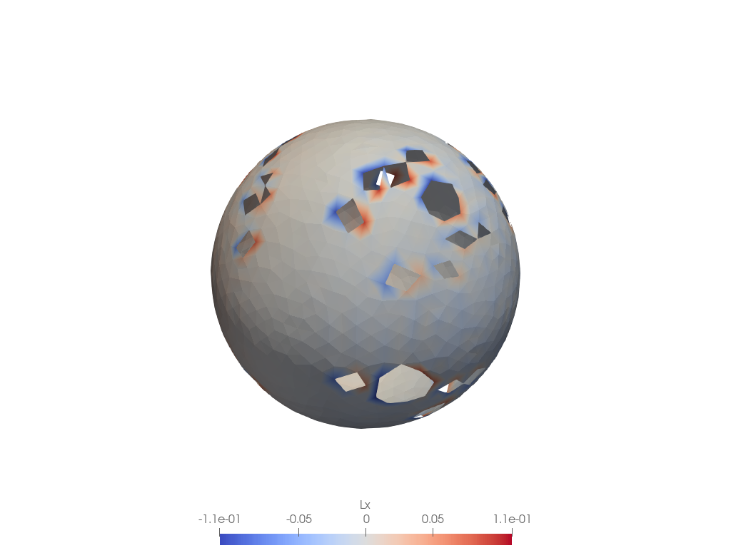
The x-coordinate is harmonic in the plane (Δx = 0), so on a flat mesh L · x would be zero everywhere. On the curved sphere it is not: L · x picks up a smooth dipole pattern aligned with the ±x axis — it is, up to the mass-matrix scaling, the x-component of the mean-curvature normal. The near-zero band around the equator and the sign flip between the +x and −x caps are the operator correctly reporting "how much does the coordinate field deviate from its local surface average." The small per-triangle speckle is marching-cubes tessellation noise (the same coarse-mesh effect discussed on the curvature page); the fixture is the same remeshed sphere. Reproducible via scripts/make_doc_images.sh.

Known limitations

• Barycentric mass, not mixed-Voronoi. Meyer et al. 2003 propose a mixed-area scheme that switches to the Voronoi region around vertex i when the incident triangle at i is non-obtuse at i, and to a truncated Voronoi (area / 4 or area / 2 depending on which angle is obtuse) otherwise. This is more accurate near obtuse triangulations and is a documented follow-up. The barycentric form FOSSIL ships is sufficient for all current downstream consumers (smoothing §2.3, curvature §2.4) on the well-conditioned triangulations produced by sanitize and isotropic remeshing.
• Obtuse triangles produce negative off-diagonals. When one angle exceeds π/2, its cotangent is negative, which means at least one L_ij < 0. The matrix is no longer "weakly diagonally dominant" in the M-matrix sense. The constant-kernel still holds (because the diagonal post-pass enforces it), and most downstream geometry uses are robust to it, but iterative solvers (when §2.2 lands) may converge slower. The fix is the mixed-area Voronoi mass above, which is designed to make the effective operator M⁻¹ L an M-matrix.
• Boundary vertices. FOSSIL targets closed solids, so boundary handling is not a first-class concern. On open meshes (e.g. an STL with one facet deleted), boundary vertices have a one-sided cotangent sum and the operator is not symmetric on the boundary subset. This is the standard cot-Lapl behaviour and matches libigl's.

See also

• mesh smoothing — the implicit smoothing variant solves (M − τL) V_new = M V; shipped variants (explicit, Taubin) use a different Laplacian (uniform weights, not cotangent) for stability reasons.
• per-vertex curvature — mean curvature is literally H_i n_i = (1/2) M⁻¹ (L V)_i, so this page is its direct prerequisite.
• csr_matrix_t — the CSR container returned by cotangent_laplacian. Has get(i,j), matvec(x, y), get_nrows(), get_nnz().
• Constants — LAPL_STATUS_*.

References

• Pinkall & Polthier, Computing discrete minimal surfaces and their conjugates, Experimental Mathematics 2(1), 1993. The original cotangent formula.
• Meyer, Desbrun, Schröder & Barr, Discrete differential-geometry operators for triangulated 2-manifolds, VisMath 2003. The mixed-Voronoi mass and the obtuse-triangle robustness story.
• Crane, Discrete Differential Geometry: An Applied Introduction, SIGGRAPH course notes 2013–2023. The canonical pedagogical reference; the FOSSIL builder follows Crane's algorithmic skeleton.
• Botsch, Kobbelt, Pauly, Alliez & Lévy, Polygon Mesh Processing, A K Peters 2010, Chapter 3. The book-length treatment, including the CSR-storage discussion that informed the FOSSIL implementation.