k=0 mesh construction

The k=0 layer is the body-conforming surface from which the volume is extruded. In the cubed-sphere topology it is assembled in two stages:

1. Cap k=0 seed — gnomonic projection of a flat square at each pole.
2. Equator k=0 — great-circle meridians from south seam to north seam, with first/last interval pinned to the cap-edge step at every seam vertex (per-j C1 spacing match).

Both stages use the Projector for ray-casting. The result is a single (ni, nj, 3) lat-lon-style structured layer split into 6 sub-arrays for the 6 blocks (4 equatorial sub-blocks + 2 caps).

Cap k=0 seed: gnomonic flat-square projection

A flat diamond is placed in the tangent plane at each cap pole, with its four corners on the cardinal axes at distance h = tan(theta_cap):

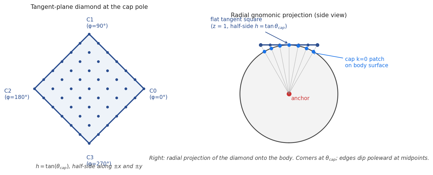
Left panel — the diamond is parametrised by (a, b) ∈ [0, 1]² with the four corners at azimuths {0°, 90°, 180°, 270°} (aligned with the 4 sub-block junctions). Bilinear interpolation gives the tangent- plane positions:

$$x_{\text{local}}(a,b)=h(1-a-b),y_{\text{local}}(a,b)=h(a-b),$$

with z_local = 1. The 4 corners lie at world-space azimuths 0°, 90°, 180°, 270°; on a unit sphere the post-projection corners sit at colatitude theta_cap exactly.

Right panel — every tangent-plane node is radially projected through the anchor onto the body via Projector.project. The projected patch is curved (it follows the body), but its index structure is the flat (nc, nc) of the diamond.

Why a diamond and not an axis-aligned square?

The four sub-block junctions on the seam parallel sit at azimuths {0°, 90°, 180°, 270°}. An axis-aligned square would put corners at {±45°, ±135°} — a 45° offset from the junctions. Rotating the square 45° (turning it into a diamond) places its corners exactly on the sub-block junctions, satisfying _overwrite_cap_boundaries's contract without any reconciliation step.

j_spacing inheritance

The 1D coordinates u_lin, v_lin ∈ [-h, +h] use the user-chosen j_spacing law (uniform or tanh2). The 4 cap edges then have a node distribution governed by that law, and because the cap edges become the equator's pole rows by DIRICHLET binding, the equator inherits the same j-distribution at the seam without further reconciliation.

from shore.surface.cap import build_cap_k0

cap_north = build_cap_k0(
    theta_cap=np.pi / 6,    # 30°
    nc=16,                   # = nj // 4 + 1
    pole="north",
    projector=body.projector,
    j_spacing="uniform",     # or "tanh2"
    j_beta=3.0,
)

Equator k=0: great-circle meridians

After both cap k=0 layers exist, their seam rings (4 cap edges concatenated in sub-block order, dropping shared corners) are extracted into (nj, 3) rings — one for the south cap, one for the north cap. Then for each j ∈ [0, nj):

1. Slerp from seam_south[j] to seam_north[j] along the great-circle meridian determined by their two unit directions.
2. Ray-cast each interior slerp position through the projector to land on the body.
3. The seam rows themselves are bit-exact copies of the cap edges (no projector round-trip needed; this preserves cap-equator conformity to floating-point precision).

The slerp parameter for each meridian is set by the constrained-distribution helper so the first/last interval matches the cap-edge first cell at the seam.

Per-j C1 seam pinning

At each seam vertex three multi-block edges meet: two cap-seam edges and one equator meridional edge. The multi-block edge spacing rule says all three first-cells must share one length:

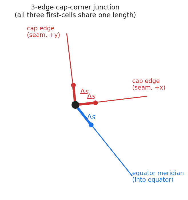
The two cap-seam edges have their first-cell length fixed by the gnomonic-square geometry — the great-circle arc between adjacent seam nodes. To match, the equator's meridional first cell at column j must equal that same arc length:

$$\mathrm{\Delta }{s}_{\text{eq}}(j)=\text{arccos}({\hat{u}}_{\text{seam}}(j)\cdot {\hat{u}}_{\text{seam}}(j+1)).$$

The equator's i-coords are colatitudes, not arc lengths, so we convert per-j by

$$\mathrm{\Delta }{\theta }_{\text{first}}(j)=\mathrm{\Delta }{s}_{\text{eq}}(j)\cdot \frac{{\text{interval}}_j}{{\omega }_j},$$

where interval_j is the colatitude span and omega_j is the anchor- angle subtended by the meridian. On a sphere with anchor at origin, interval_j ≈ omega_j and the conversion is essentially 1:1; the formula keeps the result exact for any body shape.

The interior ni − 2 cells are then graded by i_spacing on the remaining interval — implemented in shore.surface.equator._constrained_distribution.

Compatibility window and fallback

Pinning is stable only when the cap's first-cell length and the equator's natural first interval differ by less than ~2x:

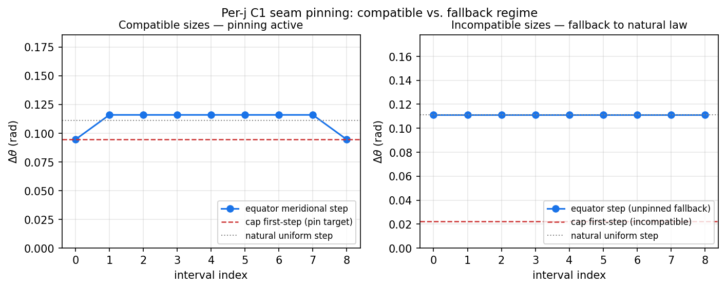
• Left (compatible): cap step (red dashed) sits within ~2x of the natural step (gray dotted). The interior absorbs the small residual smoothly. Pinning is active for all j.
• Right (incompatible): cap step is much smaller than the natural step. Pinning would force a sharp interior cell-size jump that destabilises hyperbolic marching. The equator falls back to the unpinned i_spacing law and emits a single UserWarning per build.

Rule of thumb — for compatible pinning with i_spacing='uniform':

$$\frac{{\theta }_{\text{cap}}}{n_c-1}\approx \frac{\pi -2{\theta }_{\text{cap}}}{n_i-1},n_c=\frac{n_j}{4}+1.$$

The defaults --ni 40 --nj 60 --theta-cap π/6 land inside this window.

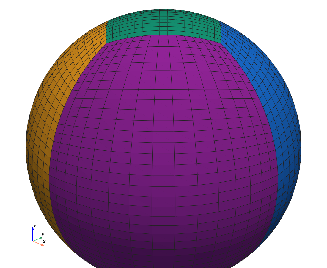
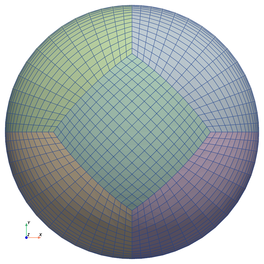
Final 6-block layout

CubedSphereTopology.build allocates a single contiguous ring array of shape (ni, ring_nj, nk, 3) for the 4 equatorial sub-blocks, with ring_nj = 4·(nc-1) + 1. Each sub-block is a numpy view into a 90° slice of this ring. Adjacent sub-blocks share their j_hi/j_lo columns by memory aliasing (SHARED face BC) — no reconciliation is ever needed at the sub-sub seams because the data is the same.

The cap blocks live in their own (nc, nc, nk, 3) arrays. Their boundaries are bound to the sub-block pole rows via DIRICHLET face BCs; _overwrite_cap_boundaries writes the sub-block pole rows into the cap edges at every layer, keeping cap-equator conformity exact.

See also

• Surface projection — the ray-casting kernel
• Hyperbolic marching — what happens after k=0
• Seam-aware normals — keeping spacing continuous during marching
• Cubed-sphere topology — block layout + connectivity
• shore.surface.cap and shore.surface.equator (Python API)