3. More data

The solver now advances the temperature by 20 explicit time steps, and computes the heat flux, minus the gradient of the temperature:

subroutine step(t)
!< Advance the temperature by one explicit time step of the heat equation; the walls stay at 0.
real(R8P), intent(inout) :: t(:,:,:)

t(2:n-1,2:n-1,2:n-1) = t(2:n-1,2:n-1,2:n-1) + dt/h**2*(t(1:n-2,2:n-1,2:n-1) + t(3:n,2:n-1,2:n-1) + &
                                                        t(2:n-1,1:n-2,2:n-1) + t(2:n-1,3:n,2:n-1) + &
                                                        t(2:n-1,2:n-1,1:n-2) + t(2:n-1,2:n-1,3:n) - 6*t(2:n-1,2:n-1,2:n-1))
endsubroutine step

subroutine heat_flux(t, qx, qy, qz)
!< The heat flux, minus the gradient of the temperature (centred differences, 0 on the walls).
real(R8P), intent(in)  :: t(:,:,:)
real(R8P), intent(out) :: qx(:,:,:), qy(:,:,:), qz(:,:,:)

qx = 0 ; qy = 0 ; qz = 0
qx(2:n-1,:,:) = -(t(3:n,:,:) - t(1:n-2,:,:))/(2*h)
qy(:,2:n-1,:) = -(t(:,3:n,:) - t(:,1:n-2,:))/(2*h)
qz(:,:,2:n-1) = -(t(:,:,3:n) - t(:,:,1:n-2))/(2*h)
endsubroutine heat_flux

The file gets more than the temperature:

error = a_vtk_file%initialize(format='raw', filename='heat.vtr', mesh_topology='RectilinearGrid', &
                              nx1=1, nx2=n, ny1=1, ny2=n, nz1=1, nz2=n, compressor='zlib')
! global data: the time and the cycle of the solution
error = a_vtk_file%xml_writer%write_fielddata(action='open')
error = a_vtk_file%xml_writer%write_fielddata(data_name='TIME', x=time)
error = a_vtk_file%xml_writer%write_fielddata(data_name='CYCLE', x=int(cycle - 1, I8P))
error = a_vtk_file%xml_writer%write_fielddata(action='close')
error = a_vtk_file%xml_writer%write_piece(nx1=1, nx2=n, ny1=1, ny2=n, nz1=1, nz2=n)
error = a_vtk_file%xml_writer%write_geo(x=x, y=x, z=x)
! the arrays ParaView colours by and draws arrows of, by default
error = a_vtk_file%xml_writer%write_dataarray(location='node', action='open', scalars='temperature', vectors='heat_flux')
error = a_vtk_file%xml_writer%write_dataarray(data_name='temperature', x=t, one_component=.true.)
error = a_vtk_file%xml_writer%write_dataarray(data_name='heat_flux', x=qx, y=qy, z=qz)
error = a_vtk_file%xml_writer%write_dataarray(location='node', action='close')
error = a_vtk_file%xml_writer%write_piece()
error = a_vtk_file%finalize()

• Field data belong to the whole dataset, not to points or cells: the time and the cycle of the solution, written right after initialize. Any kind and rank-1 arrays, strings too.
• Vectors: write_dataarray with x, y, z writes a 3-component array, here the heat flux at each point.
• Active arrays: scalars='temperature' and vectors='heat_flux' tell readers which arrays to use by default, to colour the dataset and to draw arrows.

heat_3.f90

program heat
!< Tutorial, chapter 3: the solution after 20 time steps, with the heat flux, the time and the active arrays.
use penf, only : I4P, I8P, R8P
use vtk_fortran, only : vtk_file
implicit none
integer(I4P), parameter :: n=24
real(R8P),    parameter :: h=1._R8P/(n - 1)  ! spacing of the points
real(R8P),    parameter :: dt=0.15_R8P*h**2  ! time step, stable for the explicit scheme
real(R8P)               :: x(n), t(n,n,n), qx(n,n,n), qy(n,n,n), qz(n,n,n)
real(R8P)               :: time
type(vtk_file)          :: a_vtk_file
integer(I4P)            :: i, j, k, cycle, error

x = [(real(i - 1, R8P)/(n - 1), i=1, n)]
do k=1, n ; do j=1, n ; do i=1, n
  t(i,j,k) = blob(x(i), x(j), x(k), [0.35_R8P, 0.4_R8P, 0.5_R8P]) + 0.6_R8P*blob(x(i), x(j), x(k), [0.7_R8P, 0.65_R8P, 0.45_R8P])
enddo ; enddo ; enddo
t(1,:,:) = 0 ; t(n,:,:) = 0 ; t(:,1,:) = 0 ; t(:,n,:) = 0 ; t(:,:,1) = 0 ; t(:,:,n) = 0
time = 0
do cycle=1, 20
  call step(t)
  time = time + dt
enddo
call heat_flux(t, qx, qy, qz)

error = a_vtk_file%initialize(format='raw', filename='heat.vtr', mesh_topology='RectilinearGrid', &
                              nx1=1, nx2=n, ny1=1, ny2=n, nz1=1, nz2=n, compressor='zlib')
! global data: the time and the cycle of the solution
error = a_vtk_file%xml_writer%write_fielddata(action='open')
error = a_vtk_file%xml_writer%write_fielddata(data_name='TIME', x=time)
error = a_vtk_file%xml_writer%write_fielddata(data_name='CYCLE', x=int(cycle - 1, I8P))
error = a_vtk_file%xml_writer%write_fielddata(action='close')
error = a_vtk_file%xml_writer%write_piece(nx1=1, nx2=n, ny1=1, ny2=n, nz1=1, nz2=n)
error = a_vtk_file%xml_writer%write_geo(x=x, y=x, z=x)
! the arrays ParaView colours by and draws arrows of, by default
error = a_vtk_file%xml_writer%write_dataarray(location='node', action='open', scalars='temperature', vectors='heat_flux')
error = a_vtk_file%xml_writer%write_dataarray(data_name='temperature', x=t, one_component=.true.)
error = a_vtk_file%xml_writer%write_dataarray(data_name='heat_flux', x=qx, y=qy, z=qz)
error = a_vtk_file%xml_writer%write_dataarray(location='node', action='close')
error = a_vtk_file%xml_writer%write_piece()
error = a_vtk_file%finalize()
print '(A,I0,A,ES10.3,A,F6.3)', 'heat.vtr: cycle ', cycle - 1, ', time ', time, ', maximum temperature ', maxval(t)
contains
  subroutine step(t)
  !< Advance the temperature by one explicit time step of the heat equation; the walls stay at 0.
  real(R8P), intent(inout) :: t(:,:,:)

  t(2:n-1,2:n-1,2:n-1) = t(2:n-1,2:n-1,2:n-1) + dt/h**2*(t(1:n-2,2:n-1,2:n-1) + t(3:n,2:n-1,2:n-1) + &
                                                          t(2:n-1,1:n-2,2:n-1) + t(2:n-1,3:n,2:n-1) + &
                                                          t(2:n-1,2:n-1,1:n-2) + t(2:n-1,2:n-1,3:n) - 6*t(2:n-1,2:n-1,2:n-1))
  endsubroutine step

  subroutine heat_flux(t, qx, qy, qz)
  !< The heat flux, minus the gradient of the temperature (centred differences, 0 on the walls).
  real(R8P), intent(in)  :: t(:,:,:)
  real(R8P), intent(out) :: qx(:,:,:), qy(:,:,:), qz(:,:,:)

  qx = 0 ; qy = 0 ; qz = 0
  qx(2:n-1,:,:) = -(t(3:n,:,:) - t(1:n-2,:,:))/(2*h)
  qy(:,2:n-1,:) = -(t(:,3:n,:) - t(:,1:n-2,:))/(2*h)
  qz(:,:,2:n-1) = -(t(:,:,3:n) - t(:,:,1:n-2))/(2*h)
  endsubroutine heat_flux

  pure function blob(x, y, z, centre) result(t)
  !< A hot blob: a Gaussian bump of temperature 1 at its centre.
  real(R8P), intent(in) :: x, y, z, centre(3)
  real(R8P)             :: t

  t = exp(-((x - centre(1))**2 + (y - centre(2))**2 + (z - centre(3))**2)/0.04_R8P)
  endfunction blob
endprogram heat

Running it

$ heat
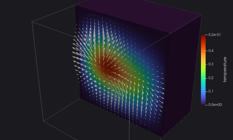
heat.vtr: cycle 20, time  5.671E-03, maximum temperature  0.518

The temperature on a cut of the cube, with the heat flux flowing out of the blobs:

What you learned

write_fielddata for global values, write_dataarray(x, y, z) for vectors, the active arrays chosen when opening the data. Reference: Field data, Active arrays.

Next: 4. A time series.