Cookbook
One task per recipe: the script (or program), and the plot it writes. The scripts read the logs of the tutorial solver, run.dat and run.csv, and a few small files; run any of them with foresight SCRIPT. Every plot here is regenerated from its recipe by scripts/docs_examples.sh and checked by the CI.
Data and columns
Two columns of a file
set terminal svg size 560,320; set output 'cb_columns.svg'
plot 'run.dat' using 1:5 with lines title 'cd'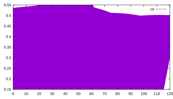
A single column
set terminal svg size 560,320; set output 'cb_single_column.svg'
# one column: x is the point number, as using 0:1
plot 'single.dat' with linespoints pt 7
With one column, x is the point number, as using 0:1; using 2 alone does the same for column 2.
One point every N
set terminal svg size 560,320; set output 'cb_every.svg'
set logscale y
plot 'run.dat' u 1:2 every 10 with linespoints pt 6 title 'every 10th iteration'
every I:J:K:L:M:N is gnuplot's full form: point and block increments, first and last points and blocks.
One dataset of a file
set terminal svg size 560,320; set output 'cb_index.svg'
set key bottom right
plot 'probes.dat' index 0 with lp pt 5 title 'run 1', '' index 1 with lp pt 9 title 'run 2'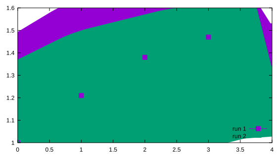
Two blank lines separate datasets; index N (0-based) picks one.
Scale and shift columns
set terminal svg size 560,320; set output 'cb_expression.svg'
set xlabel 'time [min]'; set ylabel 'cd [counts]'
plot 'run.dat' using ($1 * 0.5 / 60):($5 * 1e4) title 'cd'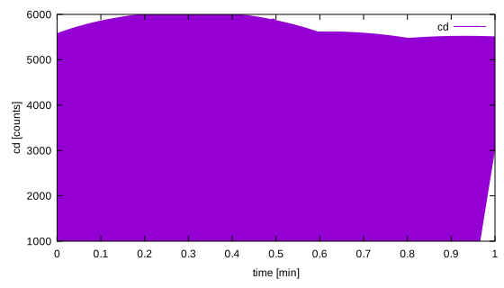
A parenthesized field is an expression evaluated per row: $N is column N, $0 the point number.
Keep only some points
set terminal svg size 560,320; set output 'cb_filter.svg'
# 1/0 is undefined: those points are gaps
plot 'run.dat' using 1:($5 > 0.3 ? $5 : 1/0) with points pt 7 title 'cd above 0.3'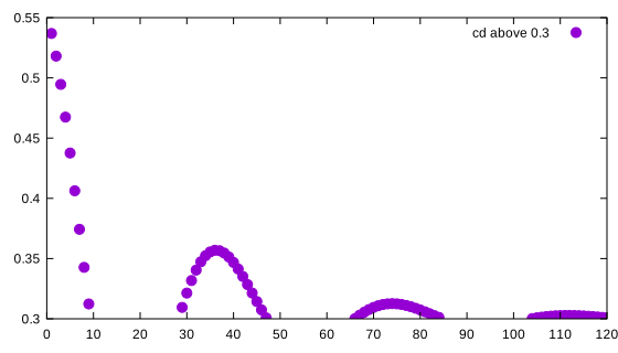
1/0 is undefined: the point is dropped, a gap in a line.
CSV with a header row
set terminal svg size 560,320; set output 'cb_csv_header.svg'
set datafile separator comma
set logscale y
plot 'run.csv' using "iteration":"continuity" title columnhead, '' using 1:"energy" title columnhead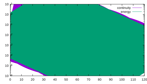
Quoted names select columns by header; title columnhead titles with the header of the y column. set key autotitle columnhead does it for every item.
Axes, ticks and key
A log axis with exponent labels
set terminal svg size 560,320; set output 'cb_logscale.svg'
set logscale y
set format y '%.0e'
set grid
plot 'run.dat' u 1:2 t 'continuity'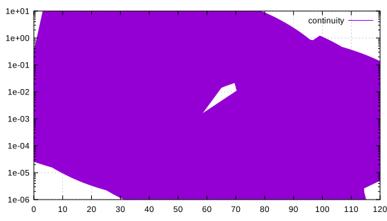
A reversed axis
set terminal svg size 560,320; set output 'cb_reversed.svg'
# min > max reverses the axis
set xrange [120:0]
plot 'run.dat' u 1:5 t 'cd'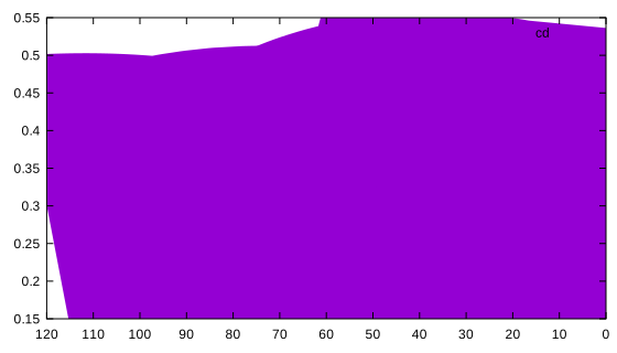
Tick steps and label formats
set terminal svg size 560,320; set output 'cb_ticks.svg'
set xtics 0,30,120
set ytics 0.1
set format y '%.2f'
plot 'run.dat' u 1:5 t 'cd'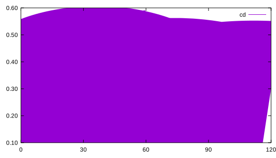
On a log axis the step is a factor: set ytics 10 puts a tick every decade.
Two y axes
set terminal svg size 560,320; set output 'cb_y2.svg'
set logscale y; set ytics nomirror; set y2tics
plot 'run.dat' u 1:2 t 'residual', '' u 1:5 axes x1y2 t 'cd'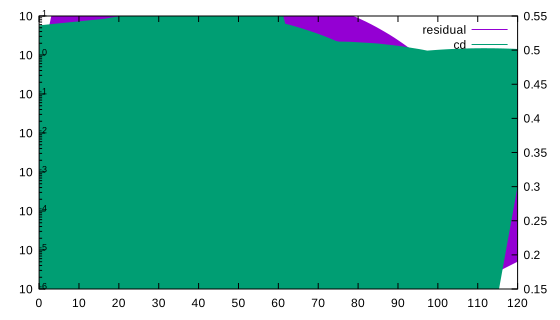
The key below the plot
set terminal svg size 560,320; set output 'cb_key.svg'
set key below box
set logscale y
plot 'run.dat' u 1:2 t 'continuity', '' u 1:3 t 'momentum', '' u 1:4 t 'energy'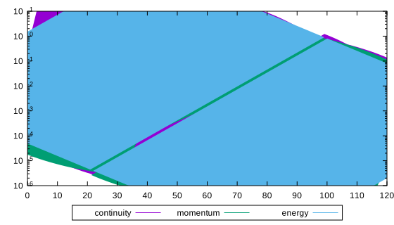
outside moves the key to the right margin (or outside left, outside top center, ...); below and above lay it out in rows.
No key
set terminal svg size 560,320; set output 'cb_no_key.svg'
unset key
plot 'run.dat' u 1:5, '' u 1:5:6 every 10 with yerrorbars
notitle keeps one item out of the key; set key noautotitle all the untitled ones.
A grid of panels
set terminal svg size 560,420; set output 'cb_multiplot.svg'
set multiplot layout 2,1
set logscale y; plot 'run.dat' u 1:2 t 'continuity'
unset logscale y; plot 'run.dat' u 1:5 t 'cd'
unset multiplot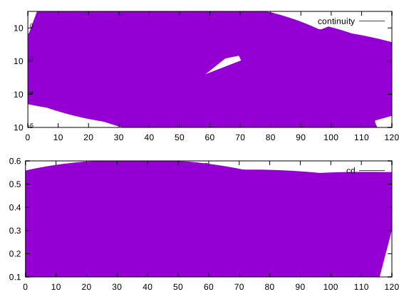
Lines, points and error bars
Line styles and point types
set terminal svg size 560,320; set output 'cb_styles.svg'
set style line 1 lc rgb '#0072b2' lw 2
set style line 2 lc rgb '#e51e10' dt 2 pt 4
set logscale y
plot 'run.dat' u 1:2 ls 1 t 'continuity', '' u 1:3 every 6 w lp ls 2 t 'momentum'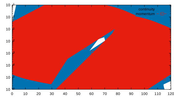
set style line N defines a style once; ls N applies it, the options after it override it.
Error bars
set terminal svg size 560,320; set output 'cb_errorbars.svg'
plot 'run.dat' using 1:5:6 every 5 with yerrorbars pt 7 ps 0.6 title 'cd'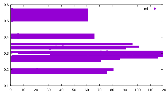
x:y:dy, or x:y:low:high; the caps keep their size under zoom.
Error bars on both axes
set terminal svg size 560,320; set output 'cb_xyerrorbars.svg'
set logscale x
set xlabel 'Re'; set ylabel 'cd'
plot 'measures.dat' using 1:2:3:4 with xyerrorbars pt 7 title 'wind tunnel'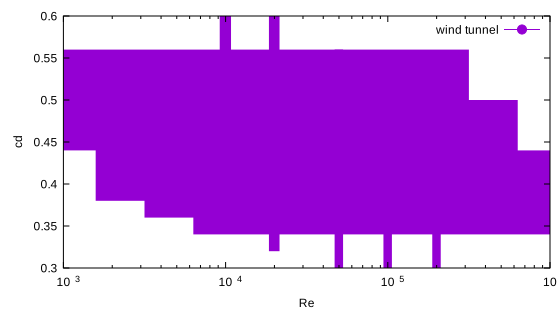
with xyerrorbars takes x:y:dx:dy, or x:y:xlow:xhigh:ylow:yhigh.
Lines through error bars
set terminal svg size 560,320; set output 'cb_errorlines.svg'
set logscale x; set xlabel 'Re'; set ylabel 'cd'
plot 'measures.dat' u 1:2:4 w yerrorlines pt 7 t 'yerrorlines', \
     ''             u 1:($2+0.1):3:4 w xyerrorlines pt 5 t 'xyerrorlines'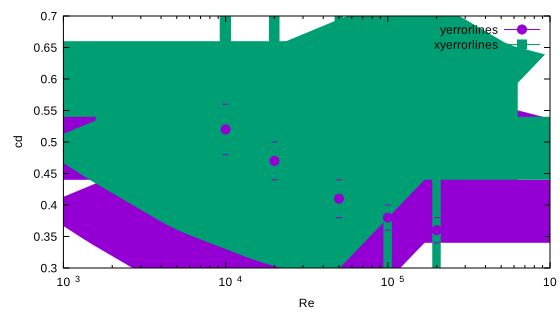
yerrorlines and xyerrorlines are linespoints with the error bars of the matching errorbars style and the same using layouts. See Lines, steps and impulses.
Steps
set terminal svg size 560,320; set output 'cb_steps.svg'
set xlabel 'iteration'; set ylabel 'dt [ms]'; set key bottom right
plot 'timestep.dat' u 1:2 w steps lw 2 t 'steps', '' u 1:2 w fsteps t 'fsteps', '' u 1:($2+1) w histeps t 'histeps + 1'
steps goes horizontally then vertically, fsteps the other way round, histeps draws a step around each point (edges halfway to the neighbours) from and back to 0. An adaptive time step reads best as steps.
A spectrum: impulses and dots
set terminal svg size 560,320; set output 'cb_impulses.svg'
set xlabel 'frequency [Hz]'; set ylabel 'amplitude'
plot 'spectrum.dat' u 1:2 w impulses lw 3 t 'impulses', '' u 1:($2+0.05) w dots t 'dots'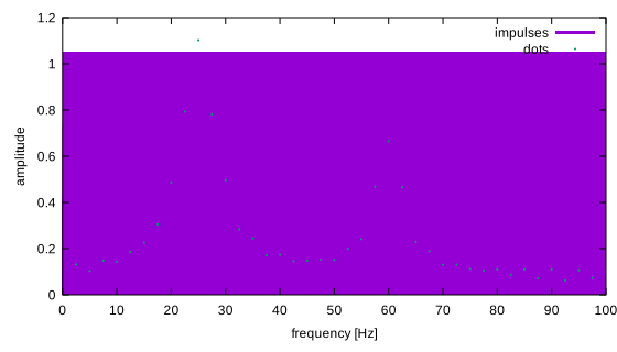
impulses draws a segment from y = 0 to each point (0 is in the autoscale, as gnuplot); dots a tiny dot per point.
Functions of x
set terminal svg size 560,320; set output 'cb_function.svg'
set samples 400
plot sin(x)/x title 'sinc', exp(-abs(x)/4) dt 2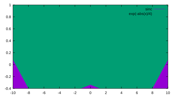
Without data, functions are sampled over [-10:10], or the xrange; set samples sets the number of points.
A model over the data
set terminal svg size 560,320; set output 'cb_model.svg'
# the function is sampled over the x range of the data
plot 'run.dat' u 1:5 with points pt 6 t 'cd', 0.30 + 0.25*exp(-x/25)*cos(x/6) t 'model'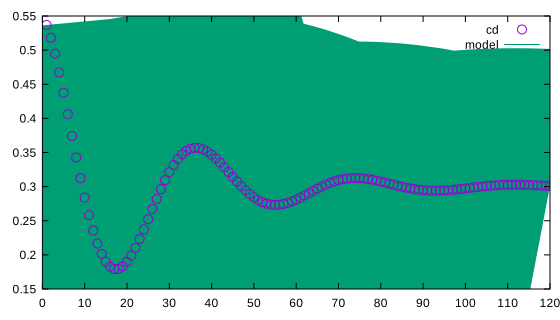
A function is sampled over the x range of the data of the same plot.
Histogram and distribution
set terminal svg size 560,320; set output 'cb_smooth.svg'
set datafile separator comma   # run.csv: the whole history in one block (run.dat breaks it at the restart)
set xlabel 'cd'; set ylabel 'iterations'; set y2label 'fraction'; set y2tics; set key top left
# bins 0.02 wide: frequency sums the 1 of each point in a bin
plot 'run.csv' u (floor($5/0.02)*0.02):(1) smooth frequency w lp pt 7 t 'histogram', \
     '' u 5:(1) smooth cnormal axes x1y2 t 'distribution'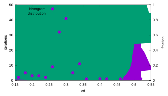
smooth frequency sums the y of the points of equal x: binned x and y = 1 count the points per bin. smooth cnormal accumulates them over the sorted x, divided by the total: the fraction of iterations below each value. smooth unique averages repeated x instead. See Smoothing.
Bars and statistics
A bar chart
set terminal svg size 560,320; set output 'cb_boxes.svg'
set style fill solid 0.5
set boxwidth 0.8 relative
plot 'run.dat' every 10 u 1:5 w boxes t 'cd every 10 iterations'
Boxes stand on y = 0 and the autoscale reaches 0 and the box edges, unlike gnuplot: bar lengths are proportional to the values. See Boxes and filled curves.
Grouped bars with category labels
set terminal svg size 560,320; set output 'cb_histograms.svg'
set style fill solid 0.6 border -1
plot 'timings.dat' u 2:xtic(1) w histograms t 'mesh', '' u 3 w hist t 'fluxes', '' u 4 w hist t 'comm'
xtic(1) labels each row with the text of column 1; the labels replace the x ticks.
Stacked bars
set terminal svg size 560,320; set output 'cb_rowstacked.svg'
set style fill solid 0.6 border -1
set style histogram rowstacked; set boxwidth 0.6
plot 'timings.dat' u 2:xtic(1) w histograms t 'mesh', '' u 3 w hist t 'fluxes', '' u 4 w hist t 'comm'
rowstacked piles the items of a row on one bar; set boxwidth 0.6 leaves room between the stacks. See Histograms.
Bars with error bars
set terminal svg size 560,320; set output 'cb_boxerrorbars.svg'
set style fill solid 0.4; set boxwidth 0.6
set ylabel 'seconds per step'
plot 'bench.dat' u 1:2:3:xtic(4) w boxerrorbars t 'mean +/- std of 20 runs'
boxerrorbars is boxes with the y error bars: x:y:ydelta, x:y:ydelta:width or x:y:ylow:yhigh:width; xtic(4) names the bars. See Box, finance and boxplot styles.
Pattern fills
set terminal svg size 560,320; set output 'cb_patterns.svg'
set style fill pattern 4 border; set key top left
plot 'timings.dat' u 2:xtic(1) w hist t 'mesh', '' u 3 w hist t 'fluxes', '' u 4 w hist t 'comm'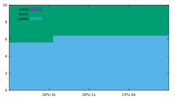
set style fill pattern N hatches the filled items, the pattern cycling from N item after item as in gnuplot: the 8 patterns of its svg terminal (0 empty, 1 and 2 crosshatches, 3 solid, 4 to 7 hatches), for prints without color.
Candlesticks and finance bars
set terminal svg size 560,320; set output 'cb_candlesticks.svg'
set boxwidth 20; set xlabel 'iteration'; set ylabel 'log10 residual'
plot 'windows.dat' u 1:2:3:4:5 w candlesticks t 'candlesticks' whiskerbars 0.5, \
     ''            u ($1+20):2:3:4:5 w financebars t 'financebars'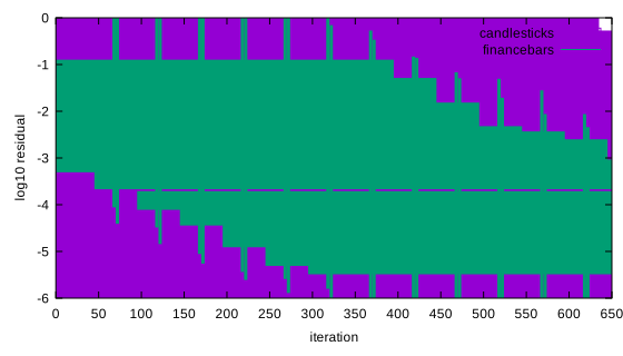
candlesticks take x:open:low:high:close (here the first, smallest, largest and last residual of each window of 50 iterations): a box between open and close, whiskers to low and high, whiskerbars 0.5 crossbars. With an empty fill a falling candle (close below open) is filled, as gnuplot: a converging run fills them all. financebars draw the same as a line with an open tick on the left and a close tick on the right.
Box plots by category
set terminal svg size 560,320; set output 'cb_boxplot.svg'
set style fill solid 0.3; set ylabel 'wall time per step [s]'
plot 'walltime.dat' u (1):2:(0.5):1 w boxplot t '12 runs per solver'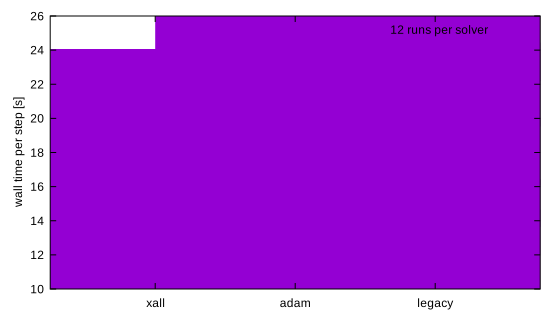
boxplot summarizes the values of its item: quartiles, median, whiskers to the farthest values within 1.5 interquartile ranges, the others as outliers. The 4th using field is a factor column: one box per solver, named on the x axis. set style boxplot sets the whisker range, outliers, sorting.
Areas and shapes
A band around a curve
set terminal svg size 560,320; set output 'cb_filledcurves.svg'
plot 'run.dat' u 1:($5-$6):($5+$6) w filledcurves fs transparent solid 0.3 t 'cd +/- dcd', \
     ''        u 1:5 w l t 'cd'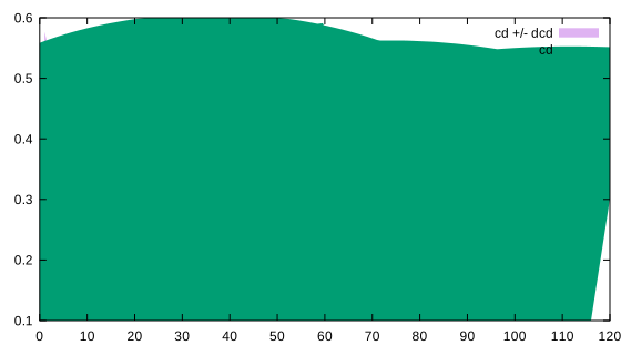
x:y1:y2 fills between two columns; filledcurves y=0 fills down to a line.
Fill above and below a line
set terminal svg size 560,320; set output 'cb_fill_above.svg'
set style fill solid 0.35; set xlabel 'iteration'; set ylabel 'cd'
plot 'run.dat' u 1:5 w filledcurves above y=0.35 t 'above 0.35', \
     ''        u 1:5 w filledcurves below y=0.35 t 'below 0.35', \
     ''        u 1:5 w l lc 'black' t 'cd'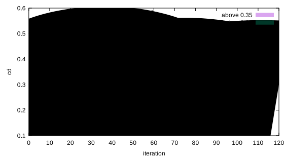
filledcurves above y=V and below y=V keep the parts of the area to the line where the curve is above or below it; x1 and x2 fill to the bottom and top of the plot, xy=X,Y to a point. The restart at iteration 60 splits the fill as it splits a line.
Rectangles
set terminal svg size 560,320; set output 'cb_boxxyerror.svg'
set style fill transparent solid 0.25
plot 'partition.dat' u 1:2:3:4:5:6 w boxxyerror t 'blocks', '' u 1:2 w p pt 7 t 'centres'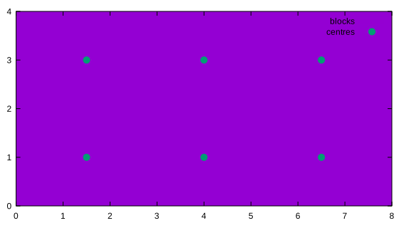
boxxyerror draws a rectangle per row, from x:y:xdelta:ydelta or x:y:xlow:xhigh:ylow:yhigh: here the blocks of a domain decomposition.
A bubble chart
set terminal svg size 560,320; set output 'cb_circles.svg'
set style fill solid 0.4
set xlabel 'cells [M]'; set ylabel 'speedup'; set xrange [0:20]; set yrange [0:11]
plot 'scaling.dat' u 2:3:4 w circles t 'memory [GB] as radius'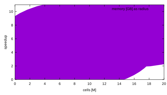
The third column is the radius, in x units. See Circles, pies and donuts.
A vector field with labelled probes
set terminal svg size 560,400; set output 'cb_vectors.svg'
set size square; set xrange [-3.5:3.5]; set yrange [-2.8:2.8]; set key below
plot 'flow.dat' every 2 u 1:2:(2*$3):(2*$4) w vectors filled head t 'velocity', \
     'probes_xy.dat' u 1:2:3 w labels left offset 1,0 point pt 7 tc 'red' notitle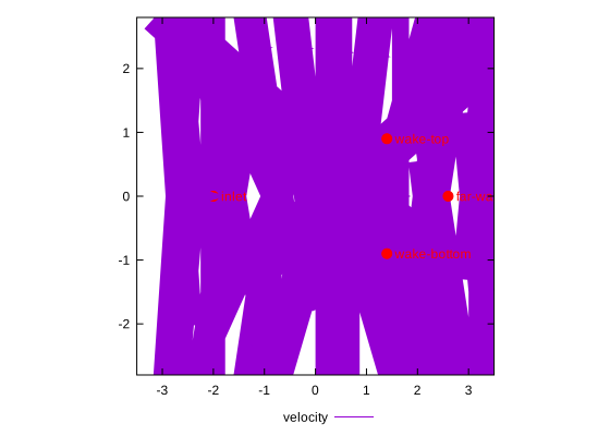
vectors draws an arrow from x:y by xdelta:ydelta (head, heads, nohead, backhead, filled); labels writes the text of a column at each point, here with its point and an offset. See Vectors, ellipses, polygons, labels and sectors. In the HTML page the heads and the labels keep their size while the zoom moves them with the data.
Arrows by length and angle
set terminal svg size 560,320; set output 'cb_arrows.svg'
set xrange [0:6]; set yrange [0:4.5]; set key below
plot 'stations.dat' u 1:2:3:4 w arrows lw 2 t 'wind (length: speed, angle: direction)', \
     ''             u 1:2:5 w labels right offset -1,0 notitle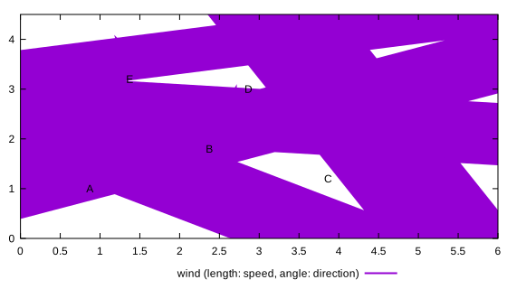
arrows takes x:y:length:angle, the length in x units and the same on the page at any angle (in degrees).
Uncertainty ellipses
set terminal svg size 560,320; set output 'cb_ellipses.svg'
set style fill transparent solid 0.2; set key top left
plot 'ellipses.dat' u 1:2:3:4:5 w ellipses t '1-sigma ellipses', '' u 1:2 w lp pt 7 t 'calibration'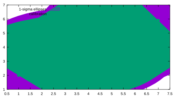
ellipses takes x:y:major:minor:angle, the diameters in x and y units, rotated on the page as gnuplot does.
Polygons from blocks
set terminal svg size 560,320; set output 'cb_polygons.svg'
set style fill solid 0.3 border; set size ratio 0.7
plot 'cells.dat' w polygons t 'cells'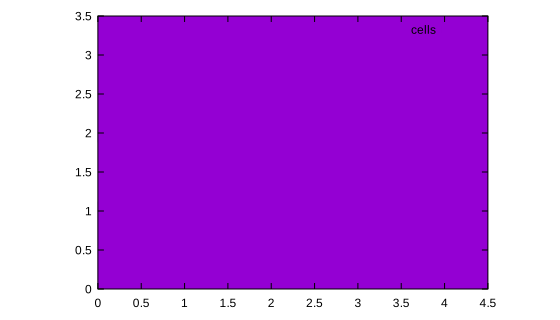
polygons closes each block of the file (blocks end at a blank line) into a polygon in the fill style: mesh cells, regions, outlines.
Heatmaps and images
A heatmap
set terminal svg size 560,400; set output 'cb_image.svg'
set cblabel 'phi'
plot 'field.dat' u 1:2:3 w image t 'phi(x,y)'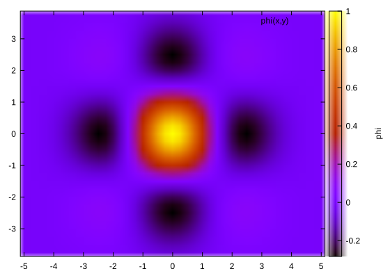
x:y:z points on a regular grid, colored by the default palette; the color box at the right.
A matrix file
set terminal svg size 560,400; set output 'cb_matrix.svg'
set palette viridis maxcolors 10
set xlabel 'sweep'; set ylabel 'block'; set cblabel 'residual'
plot 'blocks.dat' matrix w image notitle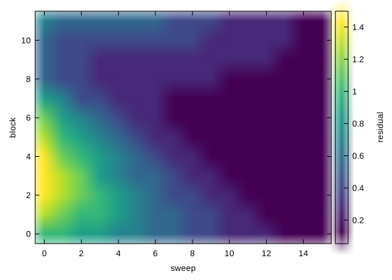
matrix reads the values as they lie in the file: columns along x, rows along y. maxcolors 10 quantizes the palette. See Images and palettes.
Palettes
set terminal svg size 760,300; set output 'cb_palettes.svg'
set multiplot layout 1,3
unset colorbox
set title 'gray'; set palette gray
plot 'field.dat' u 1:2:3 w image notitle
set title 'rgbformulae 33,13,10'; set palette rgbformulae 33,13,10
plot 'field.dat' u 1:2:3 w image notitle
set title 'defined'; set palette defined (0 'blue', 1 'white', 2 'red')
plot 'field.dat' u 1:2:3 w image notitle
unset multiplot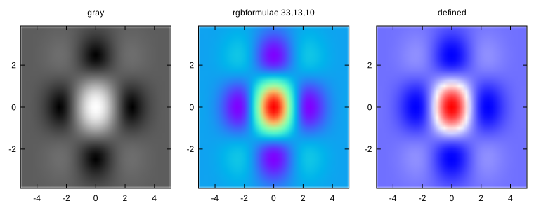
set palette gray, rgbformulae R,G,B (any of gnuplot's 37), defined (v color, ...), viridis, with negative and maxcolors N. See Images and palettes.
An RGB image
set terminal svg size 560,400; set output 'cb_rgbimage.svg'
set size ratio 0.667
plot 'wheel.dat' u 1:2:3:4:5 w rgbimage t 'rgbimage'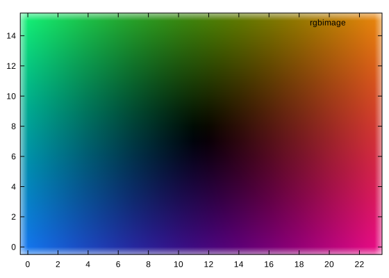
rgbimage (x:y:r:g:b) and rgbalpha (x:y:r:g:b:a) color each pixel directly, components 0 to 255 (set rgbmax 1 for fractions), without palette nor color box.
Polar and radial charts
A polar plot
set terminal svg size 520,400 theme vfd; set output 'cb_polar.svg'
set polar; set angles degrees
set size square; unset border; set border polar; unset xtics; unset ytics
set grid polar 30; set ttics 0,30; set key outside
plot 'directivity.dat' u 1:2 w lp t 'probe', 1+cos(t) t 'cardioid'
A probe's directivity against a cardioid model, theta in degrees, in gnuplot's round idiom: square plot, polar border and grid, theta labels, no x and y ticks. See Polar plots.
A wind rose
set terminal svg size 520,420; set output 'cb_windrose.svg'
set polar; set angles degrees; set theta top clockwise
set size square; unset border; set border polar; unset xtics; unset ytics
set grid polar 45; set ttics 0,45; set key outside
set style fill solid 0.6 border lc 'white'
plot 'wind.dat' u ($1-20):(0):(40):2 w sectors t '< 5 m/s', \
     ''         u ($1-20):2:(40):3 w sectors t '>= 5 m/s'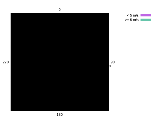
sectors draws annular sectors from azimuth:radius:angle:width, angles in the set angles unit oriented by set theta; on a polar panel they stack into a wind rose (two speed classes, one on top of the other).
A radar and a rose
set terminal svg size 480,320; set output 'cb_radar.svg'
set style fill solid 0.3
plot 'radar.dat' u 2:xtic(1) w radar t 'gpu', '' u 3 w radar t 'cpu'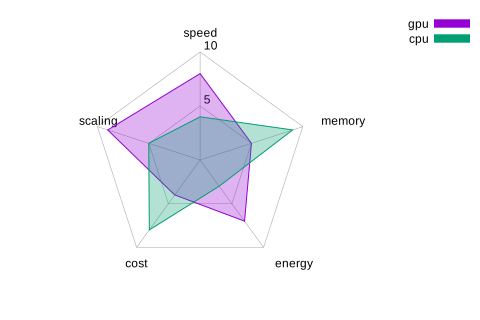
set terminal svg size 480,320; set output 'cb_rose.svg'
plot 'phases.dat' u 2:xtic(1) w rose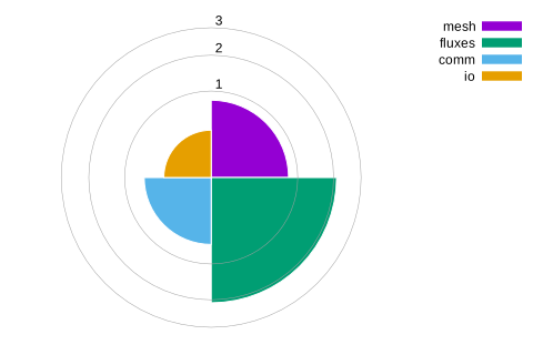
A spider plot
set terminal svg size 560,400; set output 'cb_spider.svg'
set spiderplot
set style spiderplot fs transparent solid 0.25 border lw 2
set paxis 1 range [0:10]; set paxis 2 range [0:10]; set paxis 3 range [0:10]
set paxis 4 range [0:10]; set paxis 5 range [0:10]
set paxis 1 tics 2; set grid spiderplot
plot 'solvers.dat' u 2:key(1) t 'speed', '' u 3 t 'memory', '' u 4 t 'accuracy', '' u 5 t 'scaling', '' u 6 t 'robustness'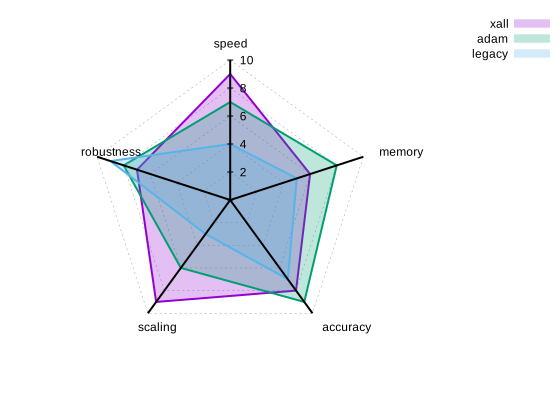
set spiderplot: each item is a radial axis, each row a polygon in its color, named by key(1); set grid spiderplot draws the web at the ticks of the first axis. foresight's with radar is the transposed shorthand (an item per polygon).
Parallel axes
set terminal svg size 560,320; set output 'cb_parallel.svg'
set paxis 1 range [0:10]; set paxis 2 range [0:10]; set paxis 3 range [0:10]
set paxis 4 range [0:10]; set paxis 5 range [0:10]; set paxis 1 tics 2
plot 'solvers.dat' u 2 w parallel lw 2 t 'speed', '' u 3 w parallel t 'memory', '' u 4 w parallel t 'accuracy', \
     ''            u 5 w parallel t 'scaling', '' u 6 w parallel t 'robustness'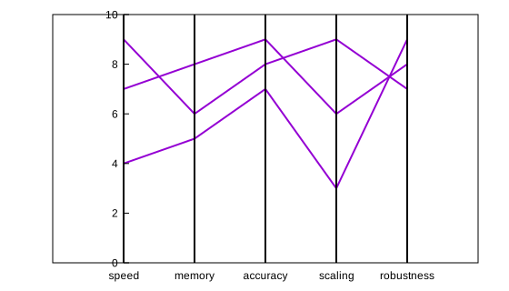
parallelaxes: each item is an axis (a column), each row a line across them; set paxis N range and set paxis N tics scale and tick each axis. See Parallel axes and spider plots.
A pie and a donut
set terminal svg size 480,320; set output 'cb_pie.svg'
set title 'Time per step'
plot 'phases.dat' u 2:xtic(1) w pie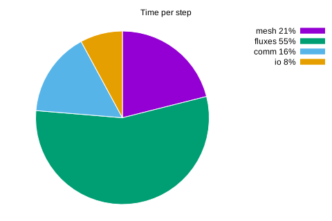
set terminal svg size 480,320 theme vfd; set output 'cb_donut_vfd.svg'
set title 'TIME PER STEP'
plot 'phases.dat' u 2:xtic(1) w pie donut 0.6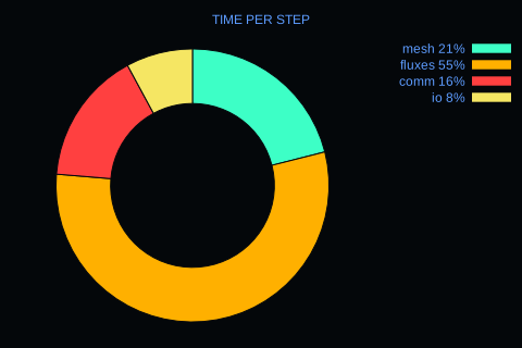
xtic(1) names the slices; the key gives their percentages.
A cluster of gauges
set terminal svg size 600,240 theme vfd; set output 'cb_gauges.svg'
plot 'run.dat' u 1 w gauge range [0:150] segments 24 format '%3.0f' t 'ITER', \
     ''        u 5 w gauge range [0:0.6] segments 24 format '%5.3f' t 'CD'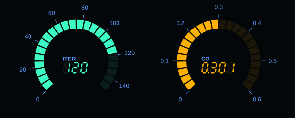
Each gauge shows the last value of its column over a fixed range, lit in cells; with --watch the needle-less gauges follow the run. See Gauges, radars and roses.
Dashboards of the 1980s
An 1980s dashboard
set terminal svg size 640,440 theme vfd; set output 'cb_vfd.svg'
set multiplot title 'RUN MONITOR'
set origin 0,0.62; set size 0.4,0.38; set readout vertical
plot 'run.dat' u 1 w readout format '%4.0f' t 'ITER', '' u 5 w readout format '%6.4f' t 'CD'
set origin 0.4,0.62; set size 0.6,0.38; set key top left
set style fill solid segments 10
plot 'timings.dat' u 2:xtic(1) w hist t 'mesh', '' u 3 w hist t 'fluxes'
set origin 0,0; set size 1,0.62; set key top right
set logscale y; set grid
plot 'run.dat' u 1:2 w l lw 2 t 'continuity', '' u 1:3 w l lw 2 t 'momentum'
unset multiplot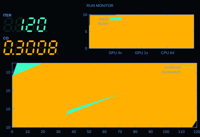
theme vfd turns the page into a vacuum fluorescent display; theme lcd into a backlit LCD. segments 10 cuts the bars into cells over the y range, the unlit ones drawn faintly. See Themes and segmented fills.
A liquid-crystal dashboard
set terminal svg size 640,300 theme lcd; set output 'cb_lcd.svg'
set multiplot layout 1,2
plot 'run.dat' u 1 w gauge range [0:150] segments 20 format '%3.0f' t 'ITER'
set key top right; set style fill solid segments 12
plot 'timings.dat' u 2:xtic(1) w hist t 'mesh', '' u 3 w hist t 'fluxes'
unset multiplot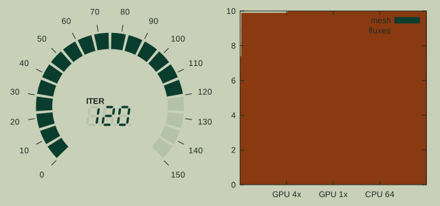
theme lcd: the pale green glass and dark segments of a backlit LCD, here with a segmented gauge and segmented bars. See Themes and segmented fills.
Seven-segment readouts
set terminal svg size 560,420; set output 'cb_readout.svg'
set multiplot title 'Run monitor'
set origin 0,0.68; set size 1,0.32
set readout horizontal
plot 'run.dat' u 1 w readout format '%4.0f' t 'ITER', '' u 2 w readout format '%9.2e' t 'CONTINUITY'
set origin 0,0; set size 1,0.68
set readout vertical top right; unset key
plot 'run.dat' u 1:5 w l t 'cd', '' u 1:5 w readout format '%6.4f' t 'CD'
unset multiplot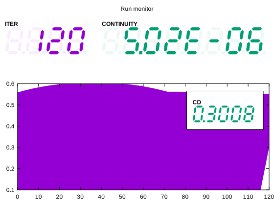
A foresight extension: the last finite value of each item in seven-segment digits, its glass fixed by the field width of format. A panel of readouts alone fills itself with digits; over a curve they lie in a window, placed as the key. See Readouts.
set terminal dumb size 72,24
set readout top right; unset key
plot 'run.dat' u 1:5 w l t 'cd', '' u 1:5 w readout format '%6.4f' t 'CD'$ foresight cb_readout_dumb.gp
0.55+----+-----+----+----+-----+----+----+-----+----+----+-----+----+
|* +----------------------+ |
0.5+ * |CD | +
| * | _ _ _ _ _ | |
| * || | _| | | | | |_| | |
0.45+ * ||_|. _| |_| |_| |_| | +
| * | | |
0.4+ * +----------------------+ +
| * |
| * |
0.35+ * ****** +
| * * ** |
| * * * ********* ***** |
0.3+ * * *** **** ************* **+
| * * ****** |
0.25+ * * +
| * * |
| * * |
0.2+ ** * +
| *** |
0.15+----+-----+----+----+-----+----+----+-----+----+----+-----+----+
0 10 20 30 40 50 60 70 80 90 100 110 120Text terminals
Text in the terminal
set terminal dumb size 64,18
plot 'run.dat' u 1:5 t 'cd'$ foresight cb_dumb.gp
0.6+--------+---------+--------+---------+--------+cd******-+
| |
|* |
0.5+* +
| * |
| * |
0.4+ * +
| * ****** |
0.3+ * ** *** ********** ********+
| * ** ********* ********* |
| ** ** |
0.2+ ** ** +
| *** |
| |
0.1+--------+---------+--------+---------+--------+---------+
0 20 40 60 80 100 120set terminal dumb writes to the standard output; set output 'plot.txt' to a file.
Unicode text in the terminal
set terminal block braille size 64,18
plot 'run.dat' u 1:5 t 'cd'$ foresight cb_block.gp
0.6⡏⠉⠉⠉⠉⠉⠉⠉⠉⠙⠉⠉⠉⠉⠉⠉⠉⠉⠉⠋⠉⠉⠉⠉⠉⠉⠉⠉⠙⠉⠉⠉⠉⠉⠉⠉⠉⠉⠋⠉⠉⠉⠉⠉⠉⠉⠉⠙cd⢉⣉⣉⣉⣉⣉⠉⡇
⣇ ⡇
⡏⢆ ⡇
0.5⡏⠙⡄ ⠈⡇
⡇ ⢣ ⡇
⡇ ⠈⡆ ⡇
0.4⡏⠁ ⢱ ⠈⡇
⡇ ⠈⡆ ⢀⠔⠒⠒⢄⡀ ⡇
0.3⣇⡀ ⢸ ⡔⠁ ⠈⠢⣀ ⢀⣀⡠⠤⠤⠤⠤⣀⣀⣀ ⢀⣀⣀⣀⣀⣀⣀⣀⡇
⡇ ⢇ ⢀⠜ ⠑⠢⠤⣀⡠⠤⠒⠊⠁ ⠉⠉⠉⠉⠉⠉⠉⠉⠁ ⡇
⡇ ⠘⡄ ⢀⠎ ⡇
0.2⣇⡀ ⠘⡄ ⡠⠊ ⢀⡇
⡇ ⠘⠢⠒⠁ ⡇
⡇ ⡇
0.1⣇⣀⣀⣀⣀⣀⣀⣀⣀⣠⣀⣀⣀⣀⣀⣀⣀⣀⣀⣄⣀⣀⣀⣀⣀⣀⣀⣀⣠⣀⣀⣀⣀⣀⣀⣀⣀⣀⣄⣀⣀⣀⣀⣀⣀⣀⣀⣠⣀⣀⣀⣀⣀⣀⣀⣀⣀⡇
0 20 40 60 80 100 120block draws with Unicode characters of 2 x 4 dots (braille), 2 x 3 (sextants), 2 x 2 (quadrants, the default) or 1 x 2 (half). Add ansi (or ansi256, ansirgb) to draw each series in its color, in dumb as well.
From Fortran
From Fortran: gaps in the data
NaN values are gaps, as gnuplot's undefined points; save writes any of the formats, - text on the standard output.
y(30:40) = ieee_value(1.0_R8P, ieee_quiet_nan)   ! a missing stretch: the line breaks there
call fig%init(width=560_I4P, height=320_I4P)
call fig%plot(x, y, title='sin(x), samples 30-40 missing')
call fig%save('cb_gaps.svg')
call fig%save('cb_gaps.html')
call fig%save('-')                                 ! text, on the standard output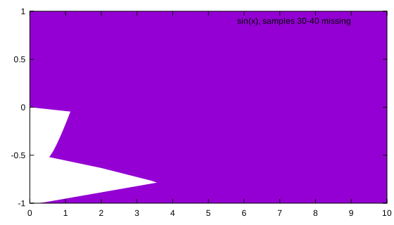
$ cb_gaps

     1+-------+------+-------+-------+------+--sin(x), samples 30-40 missing******-+
      |       *       **                                     **        *           |
      |     **          *                                    *          *          |
      |    *            **                                 **            **        |
   0.5+   **              *                               *               *        +
      |  *                 *                             *                 *       |
      | *                  *                             *                  *      |
      |*                                                *                    *     |
      |*                                               *                     **    |
     0+                                               *                        *   +
      |                                              *                          *  |
      |                                             *                            * |
      |                                            *                             * |
  -0.5+                                            *                              *+
      |                                          **                                |
      |                                         *                                  |
      |                              *         *                                   |
      |                               ***   ***                                    |
    -1+-------+------+-------+-------+------+-------+-------+------+-------+-------+
      0       1      2       3       4      5       6       7      8       9      10
From Fortran: run gnuplot commands
script_object is the interpreter of the command line: scripts and single commands from the program, with errors returned, never stopped on.
call gp%init('cb_script.svg')
call gp%run_text("set terminal svg size 560,320"//new_line('a')// &
                 "set logscale y; plot 'run.dat' u 1:2 t 'continuity', '' u 1:3 t 'momentum'", iostat, iomsg)
if (iostat /= 0) print '(A)', iomsg
call gp%execute('set key bottom left', iostat, iomsg)
call gp%execute('replot', iostat, iomsg)            ! re-reads run.dat and renders again